The Fundamental Concepts of Hypothesis Testing
A/B testing is an experimental approach that facilitates Hypothesis Testing. This process is best understood through an example.
Imagine an eCommerce site that implements a change to its item recommendation module, believing that this update will promote upsells and thereby increase Gross Merchandise Value per visitor (GMV/visitor). To evaluate the impact of this change, the site conducts an A/B test, splitting visitors into two groups: a Control group that continues to see the original recommendations module, and a Test group that experiences the updated module.
Let’s assume that the average GMV/visitor in the Control group is $100, while the Test group averages $102. At first glance, it might seem obvious that the new module led to a $2 increase in GMV/visitor, suggesting it is the better option.
Sampling Variability, Sampling Distribution and Standard Error
However, the situation is more complex—this $2 increase may have occurred by random chance.
Both the Test and Control groups are samples of the broader population of site visitors. Because of this, they are subject to sampling variability (or sampling error), meaning that even if the new recommendation module had no real effect, we might still observe a difference in GMV/visitor due to random fluctuations in who ended up in each group and what they purchased.
To illustrate how sampling variability can arise, consider the GMV/visitor for all visitors on the site over a given time period, independent of any A/B tests. Suppose during that period, there were 10,000 visitors whose GMVs ranged from $20 to $180. For simplicity, assume the GMV/visitor follows a normal distribution—a reasonable assumption in many A/B testing scenarios.
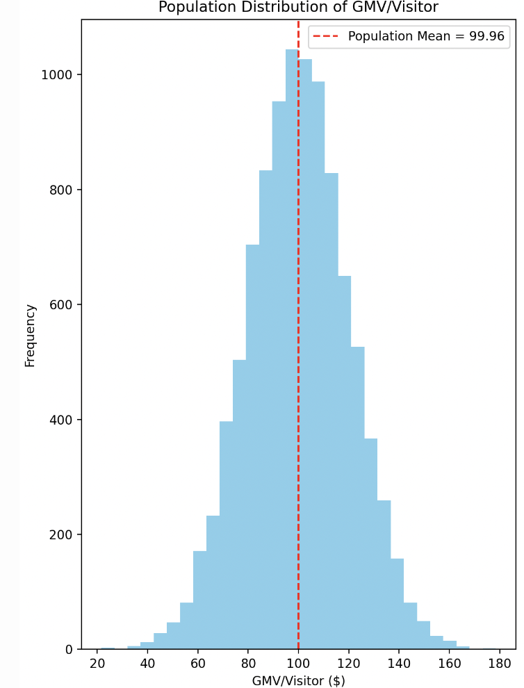
This represents the population distribution of GMV/visitor, encompassing all visitors during that time period. Now, if we randomly split these visitors into two groups, we would observe the sampled GMV/visitor for each group.
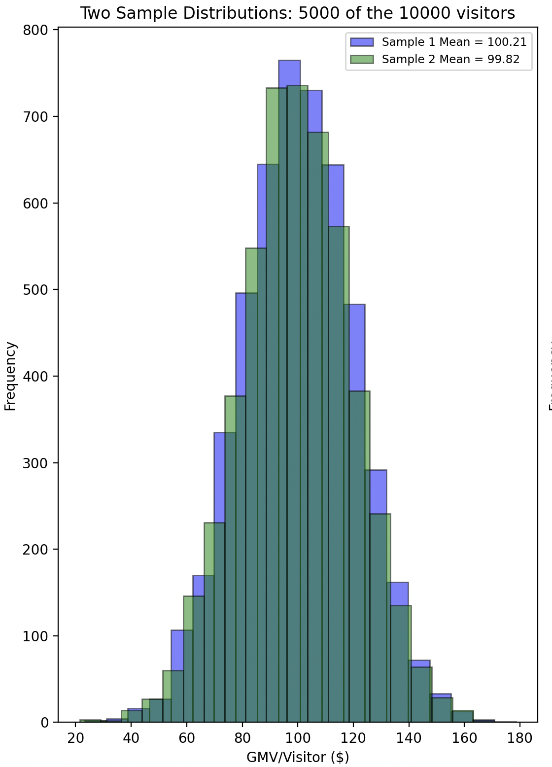
Even though both groups originate from the same population distribution, each will have its own sample distribution with different sample statistics, such as the mean, median, and standard deviation.
To further illustrate this, imagine repeating the sampling process multiple times. Even though all samples come from the same population distribution, the sample means will vary from one sample to the next due to sampling variability.
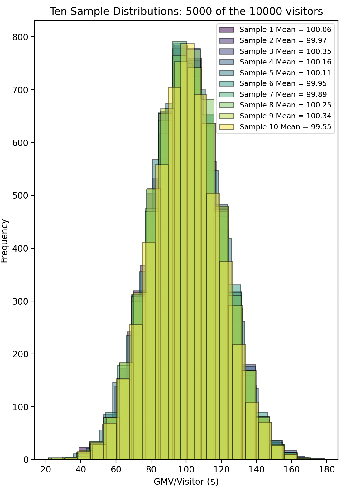
In this scenario, no A/B test was actually conducted, no changes were made, and we simply sampled from the same population distribution—yet the sample means of the groups differ by some amount purely due to chance.
Despite our best efforts to ensure that similar types of visitors are represented in both groups in similar proportions, some variability will always exist.
To clarify, there are three types of distributions at play here:
- Population Distribution: The distribution of GMV/visitor for all visitors during the time period. It has its own statistics, such as the population mean, median, and standard deviation.
- Sample Distributions: Each time we draw a sample from the population, we get a sample distribution with its own sample statistics, such as the sample mean, sample median, and sample standard deviation. These sample distributions vary due to sampling variability.
- Sampling Distribution: If we were to repeatedly take many samples from the population and calculate the sample statistic (e.g., the mean) for each sample, the distribution of these sample statistics forms the sampling distribution. For instance, the sampling distribution of the mean represents the distribution of sample means from all possible samples of a given size drawn from the population.
In A/B testing, when we compare statistics like the mean between Test and Control groups, we are not comparing the population means directly—we are comparing sample means, which are drawn from the sampling distributions of each group.
The standard error of a statistic is the standard deviation of its sampling distribution. If the statistic is the sample mean, we refer to the standard error of the sample mean.
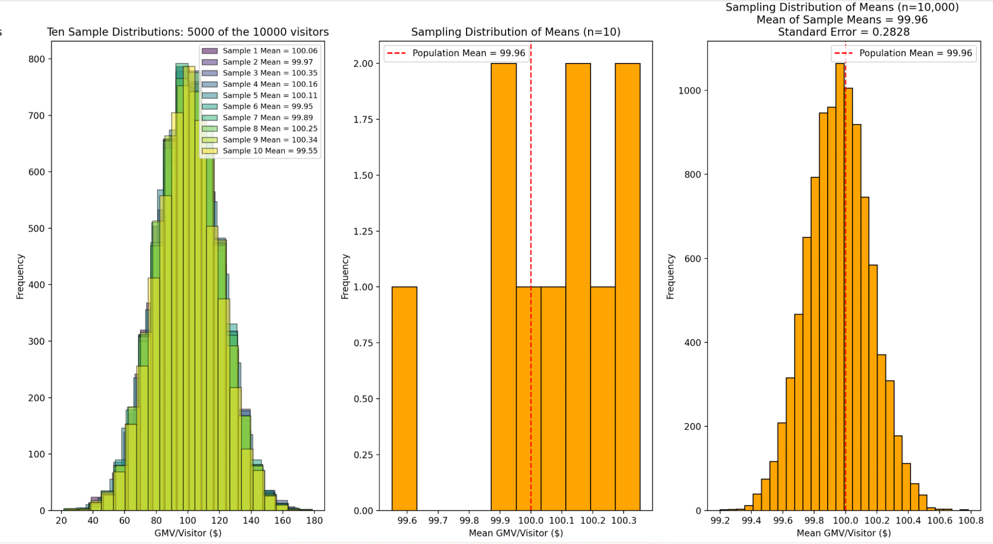
This concept is crucial because sampling variability leads to the formation of a sampling distribution, and the standard error quantifies the extent of this variability.
It is the presence of standard error that complicates drawing conclusions from an A/B test, as it means the observed difference between groups could be due to chance rather than a real effect.
Chance vs. Genuine Impact
So far, we’ve discussed how sampling variability can lead to differences in sample statistics even when there is no real effect, leading to “chance impact”. But what happens when there is a genuine impact?
When a change has a real effect, it alters the population distribution of the group exposed to the change. Before an A/B test begins, both the Control and Test groups are assumed to share the same population distribution. However, during the test, the Test group’s population distribution shifts due to the impact of the change, while the Control group’s distribution remains the same.
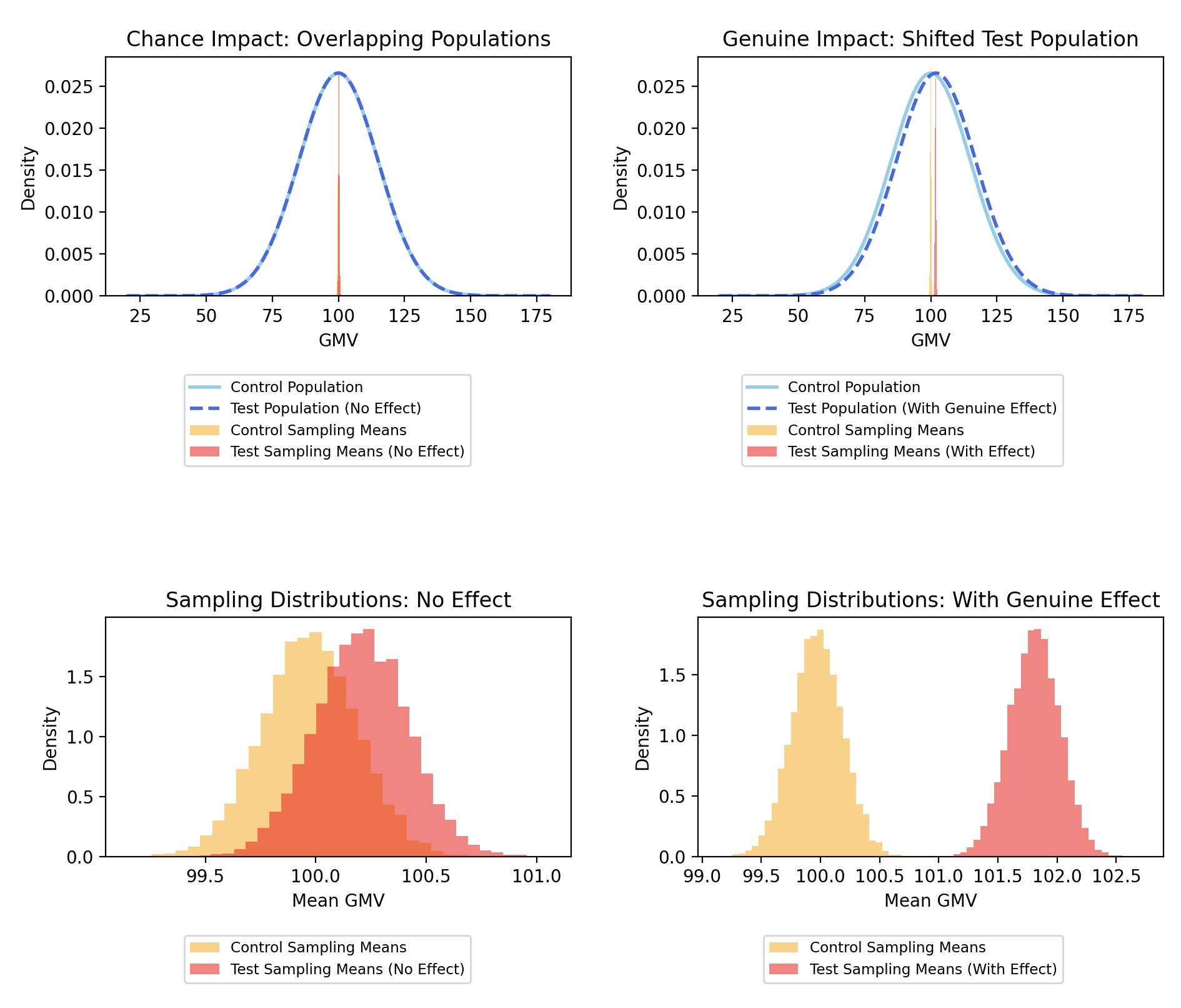
Continuing the example from earlier: initially, both the Control and Test groups have the same population distribution of 10,000 visitors with GMVs ranging from $20 to $180, though their sample distributions may differ. By the end of the test, if the new module has a genuine impact, the Test group’s population distribution (and consequently its sampling distribution) will have shifted, while the Control group’s distributions remain consistent with those observed before the test.
In summary, when we talk about genuine impact, we are referring to changes in the underlying population parameters due to the tested intervention. These population parameters are not directly observable and must be estimated from sample statistics. However, as we’ve seen, sample statistics are distributed across a sampling distribution, leading to potentially noisy comparisons.
The role of Hypothesis Testing is to determine whether the observed difference between the Test and Control groups is merely due to chance or represents a genuine effect (i.e., statistically significant).
Null Hypothesis and Alternative Hypothesis
So it looks like we are in a real pickle. We want to see if a change, such as in the item recommendations module, made a genuine impact on GMV/visitor—that is, whether it changed the population distribution of GMV/visitor. But we cannot observe both a change and its counterfactual effects on the entire population; therefore, the population must be split into samples. This, however, introduces sampling variability, making it hard to tell real impact from chance.
Hypothesis testing offers a framework to address this challenge by providing a structured approach to determine whether an observed difference between Test and Control sample statistics is likely due to chance or indicates a real effect. Specifically, under the Null Hypothesis, we assume that any observed difference is due to random sampling variability and that there is no real impact.
Our goal in hypothesis testing is to gather evidence that allows us to reject the Null Hypothesis. By demonstrating that the observed difference is too extreme to be attributed to chance alone, we indirectly support the Alternative Hypothesis, which posits that there is a genuine impact.
This process might seem counterintuitive at first. Why do we focus on rejecting the Null Hypothesis rather than directly rejecting or supporting the Alternative Hypothesis?
The reason lies in the nature of statistical inference. Unlike in formal logic, where something can be definitively proven true or false, statistical inference deals with data that is subject to sampling variability. This variability means that we can never observe every possible outcome in the population; we can only work with samples. Population parameters, such as the true mean or the true difference in means, are not directly observable. Consequently, we cannot achieve the absolute certainty that mathematical proofs require.
Instead of seeking absolute proof, we assess the likelihood of the observed data under the Null Hypothesis. If this probability is sufficiently low, we reject the Null Hypothesis.
But why focus on rejecting the Null Hypothesis and not on rejecting the Alternative Hypothesis?
Although the Null and Alternative Hypotheses are symmetrical in the sense that rejecting one lends support to the other, they are not symmetrical in terms of the burden of proof.
To reject the Null Hypothesis requires just one comparison: if the observed data is too extreme compared to what we would expect if there were no impact—which is what the Null Hypothesis assumes—we may reject the Null Hypothesis.
On the other hand, to reject the Alternative Hypothesis, which posits that some genuine impact exists, would require comparing the observed data against all possible scenarios where a genuine impact could occur. Only if the observation is too extreme for all these scenarios can we reject the Alternative Hypothesis in favor of the Null Hypothesis, effectively supporting the idea that no genuine impact exists.
This complexity makes it much more sensible to focus on rejecting the Null Hypothesis.
Central Limit Theorem and the Law of Large Numbers
In the above section, it was mentioned that in Hypothesis Testing, to establish a genuine impact, we have to show that the observed difference between Test and Control sample means is too extreme compared to what we would expect if there were no impact.
Before expanding on what that entails, let’s take a slight detour to discuss some other statistical concepts that:
- Will simplify our discussion of Hypothesis Testing
- Are widely applicable to online A/B Testing
These concepts are the Central Limit Theorem and the Law of Large Numbers.
The Central Limit Theorem (CLT) essentially guarantees that under certain conditions, the sampling distributions of the Test and Control group means will approximate a normal distribution. Interestingly, this is true even when the samples themselves or the underlying population distribution are not normal.
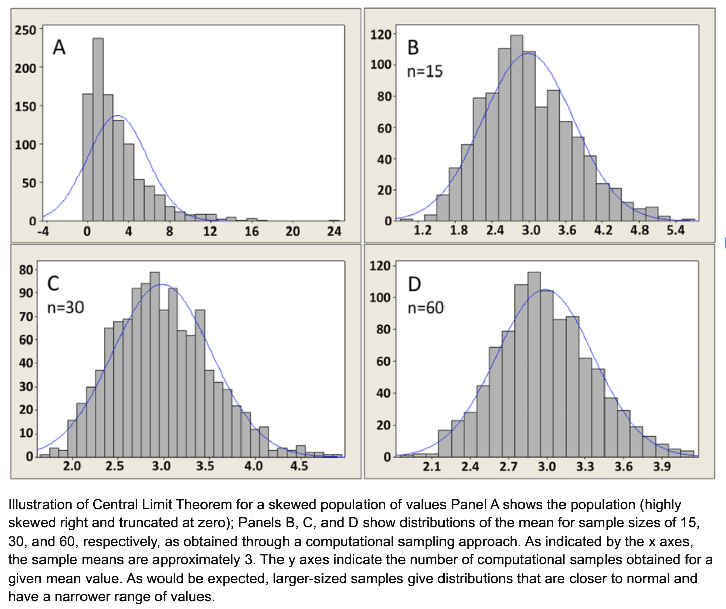
Image Source: Illustration of Central Limit Theorem for a skewed population of values
The fact that the sampling distribution of means approximates a normal distribution implies that the difference between the means of the Test and Control groups will also follow a normal distribution.
Under the Null Hypothesis, this sampling distribution of differences will be centered around zero, indicating no real effect.
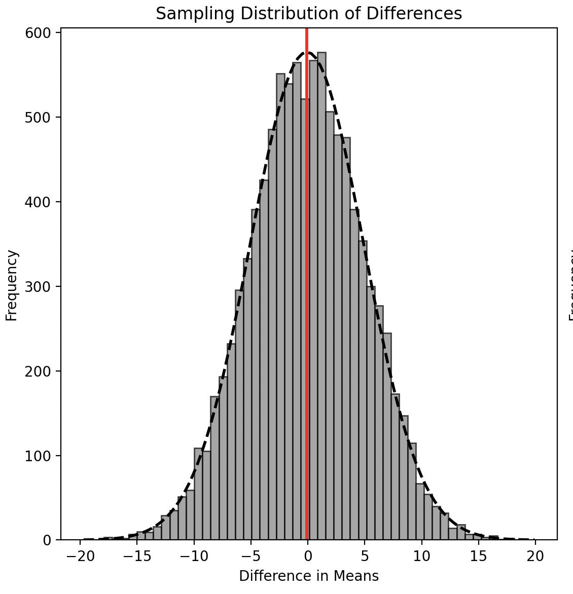
If we model the Alternative Hypothesis (as we will see in an example later), the sampling distribution of differences under it will also follow a normal distribution, but will be centered around some non-zero value, reflecting the presence of an effect.
The Law of Large Numbers (LLN), on the other hand, guarantees that under certain conditions, as the sample size increases, the sample mean converges to the population mean. This reassures us that sampling variability reduces with an increase in sample size—i.e., the sampling distribution of means becomes tighter around its center—making the comparison of observations against the Null or Alternative Hypothesis less noisy.
In other words, the LLN leads to a reduction in the standard error of the mean, thereby reducing the probability that observed differences are due to chance rather than a real effect.
Both CLT and LLN hold under the same set of assumptions:
- Sample Size: There must be a large number of samples. A common rule of thumb is that 30 samples are often sufficient for the LLN and CLT to apply. However, in the case of fat-tailed distributions like the 80/20 Pareto distribution, it can take about \(10^{14}\) samples for the LLN to take effect, and the CLT may not apply at all.
- Independence and Identically Distributed (i.i.d.) Samples: The samples must be independent and identically distributed. This means that drawing one sample does not influence any other sample, and each sample is drawn from the same distribution with the same statistical properties.
- Finite Mean and Variance: The underlying population distribution must have a finite mean and variance. The CLT does not apply to distributions like the Cauchy distribution, which has an undefined variance.
These conditions generally hold in most online A/B testing environments, where experiments usually run with at least thousands of data points. The experimentation setup ensures i.i.d. distribution of samples (to be discussed more later). The underlying distributions generally have finite means and variances, especially after outlier removal (also to be discussed later).
We have taken this detour from discussing Hypothesis Testing because, as we shall see, it is easier to illustrate the concepts of Hypothesis Testing using a normal distribution and means—situations where the CLT applies. However, it’s important to note that Hypothesis Testing concepts such as statistical significance and statistical power are general and do not inherently rely on assumptions of normality.
This distinction is crucial because while normal distributions and means are common in many online A/B testing scenarios, they are not universal. For example, when the statistic of interest is a median or percentile, the CLT does not apply. We will explore these cases after addressing the core concepts of Hypothesis Testing using normal distributions and means.
Statistical Significance and False Positives
We now return to the process of determining whether the observed difference between sample means is too extreme compared to what we would expect if there were no real impact.
In Hypothesis Testing, the rule of thumb is that any observation with less than a 5% probability of belonging to the distribution under the Null Hypothesis is considered statistically significant, suggesting a genuine impact. This is often expressed as a situation where the p-value is less than 0.05.
This means that when the Central Limit Theorem (CLT) applies and the distribution under the Null Hypothesis is normal with a mean of zero, any observation more than two standard errors away from the mean is typically considered statistically significant.
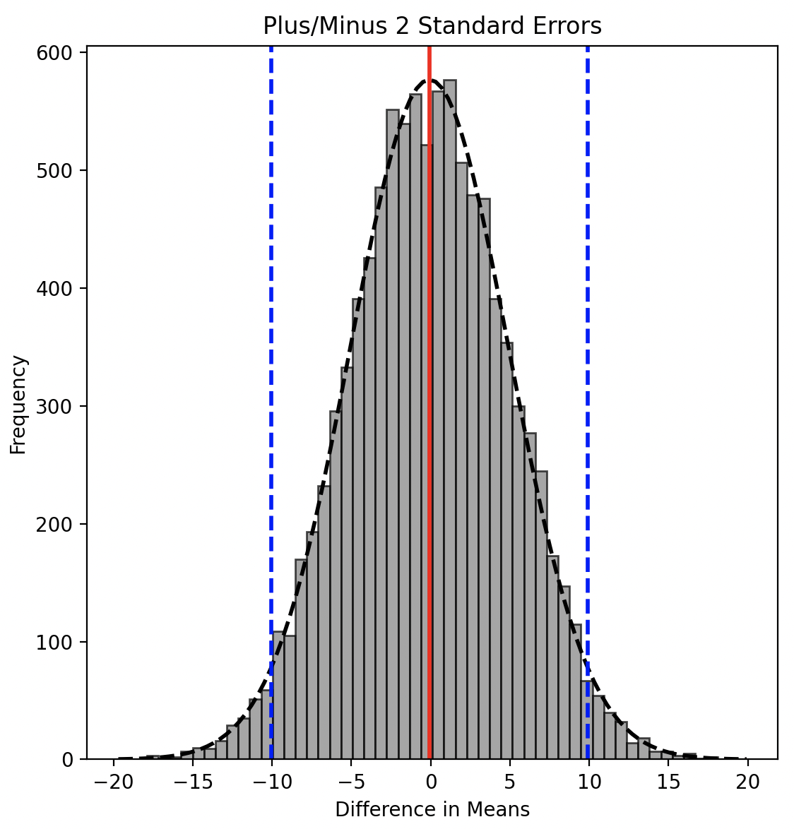
This might seem counterintuitive. After all, there is still a 5% chance that the observed difference is simply due to random chance—that is, it comes from the distribution under the Null Hypothesis.
That is correct, and such a situation is known as a False Positive or Type I error—where we mistakenly reject the Null Hypothesis and attribute the difference to a genuine impact when it is actually due to chance.
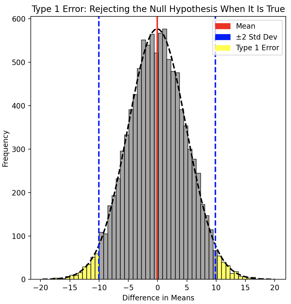
Ultimately, this 5% threshold is a convention—a balance between rigor and practicality. It is more of an art than a science, and in some cases, this threshold is lowered to reduce the risk of False Positives. However, as we will see in the next section, lowering the threshold introduces a different tradeoff.
Before moving on, it’s important to clarify a key concept: the idea of statistical significance. It’s crucial not to confuse statistical significance with practical significance.
Statistical significance relates specifically to the Null Hypothesis, while practical significance is defined in the context of the business, product, or other factors motivating the A/B test.
For instance, in the context of our item recommendations module, a $2 difference might be practically significant for the business, but not statistically significant if sampling variability is high, resulting in a high standard error. Conversely, a $0.20 difference might be statistically significant if sampling variability is low, even if it is not practically significant for the business.
False Negatives and Statistical Power
In the previous section, we introduced the concept of a False Positive or Type I error. The flip side of this is a False Negative, or Type II error, which occurs when there is a genuine impact, but we mistakenly attribute the observed result to chance, failing to reject the Null Hypothesis even though the Alternative Hypothesis is true.
Just as in the case of False Positives, the concept of False Negatives is general to Hypothesis Testing. However for simplicity, we once again lean on the CLT and normal distributions for illustration.
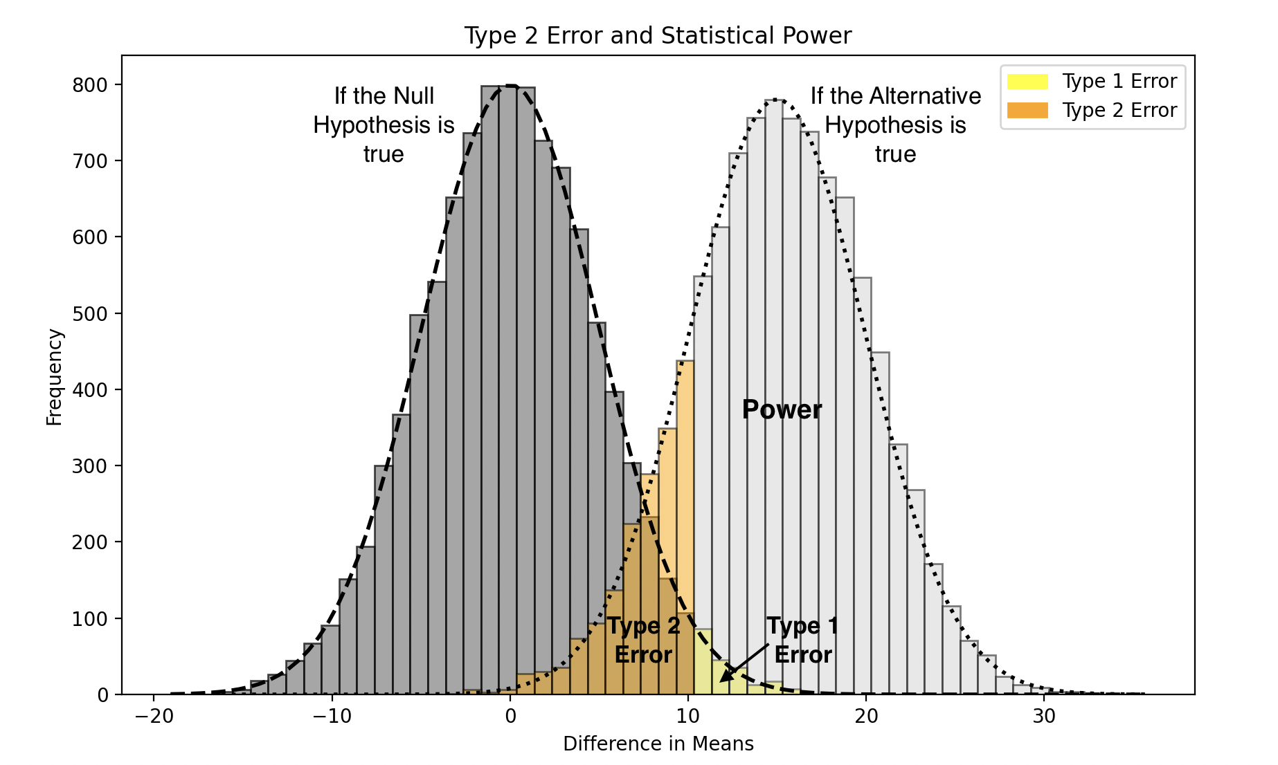
False Negatives are more likely when the difference between the means of the two distributions (i.e., the effect size) is small, the underlying population has high variability, or the sample size is low. These factors increase the overlap between the sampling distributions under the Null and Alternative Hypotheses, making it harder to detect a real effect. Additionally, choosing a lower p-value threshold can further increase the risk of False Negatives by making it more difficult to reject the Null Hypothesis.
It was mentioned in the previous section that we tolerate some False Positives by design. It may be clear by now that this is done to strike a balance against False Negatives (as indicated by the yellow stripes vs. black stripes in the chart above).
False Negatives reduce the effectiveness of testing. Therefore, during the test design phase, we focus on understanding the probability of avoiding False Negatives—a measure known as Statistical Power.
Statistical Power is calculated by modeling our desired effect size, known as the minimum detectable effect (MDE), as the center of the distribution under the Alternative Hypothesis. The overlap between this Alternative Hypothesis distribution and the Null Hypothesis distribution represents the probability of False Negatives—this probability is known as beta (β). Therefore, Statistical Power, calculated as 1 - β, represents the probability that the test will correctly detect the effect if it exists.
Understanding Statistical Power is crucial for decision-making.
For example, if the Statistical Power is low and we cannot improve it by adjusting the MDE or increasing the sample size, and the test is expensive to run, we might decide against conducting the test.
Conversely, if the test is inexpensive to run or if we can improve Statistical Power by increasing the sample size or reducing variability, we may proceed with the test.
The general convention is to aim for at least 80% Statistical Power, meaning we accept a maximum of 20% probability of False Negatives.
Often, sample size is the primary variable we can control to increase Statistical Power. This is why sample size estimation is a critical aspect of test design—it directly impacts our ability to detect genuine effects with statistical significance. We will explore how to calculate Statistical Power more concretely when we discuss z-tests.
The Direction of Tests
We have covered nearly all the essential concepts for Hypothesis Testing, with one last topic to address: the direction of tests. The direction, also known as the tail of a test, refers to whether we are interested in detecting a change that is only greater than the baseline, only less than the baseline, or if we’re interested in changes in either direction—that is, greater or less than the baseline.
For instance, a right-tailed test only assesses whether the statistic of interest (e.g., the mean of the Test group) is greater than that of the Control group. A left-tailed test, on the other hand, evaluates whether the Test statistic (e.g., mean) is less than that of the Control group. Meanwhile, a two-tailed test examines whether the Test statistic is either greater than or less than that of the Control group.
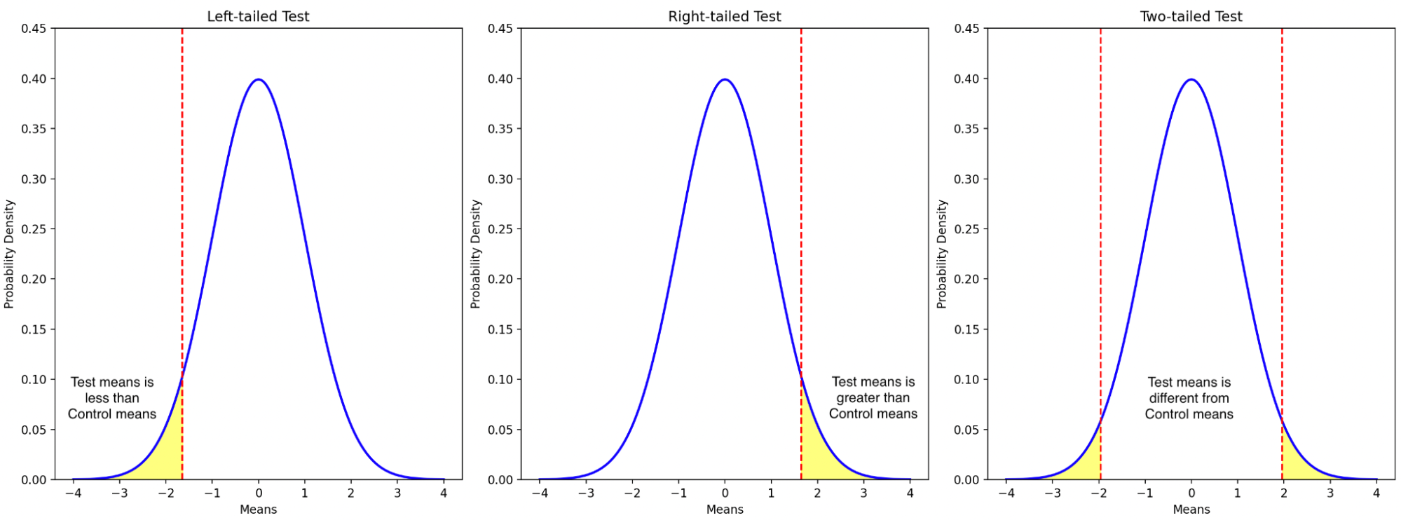
Determining the tail of a test is crucial because it affects the threshold for statistical significance, which in turn influences the statistical power of the test. In a one-tailed test (whether left-tailed or right-tailed), the entire significance level (alpha), typically 0.05, is allocated to one tail of the distribution. In contrast, a two-tailed test divides the significance level between both tails of the distribution, meaning the alpha is 0.025 in each direction. This approach is more conservative because it requires stronger evidence to reject the Null Hypothesis in either direction, ensuring the test is sensitive to deviations from the baseline in both directions. While this reduces the risk of Type I errors (false positives) in both directions, it also slightly reduces the statistical power compared to a one-tailed test when the true effect is expected in one specific direction.
Choosing between a one-tailed and two-tailed test depends on the specific hypothesis being tested and the research question at hand. If there is a strong theoretical reason to expect a change only in one direction, a one-tailed test may be appropriate. Otherwise, a two-tailed test is generally preferred to capture potential changes in either direction.
Two Sample z-test for Means
Now that we have familiarized ourselves with the most important concepts in Hypothesis Testing, we are ready to make our understanding more concrete by looking at a specific Hypothesis Test—namely, the two sample z-test for means.
As the name implies, this test assumes a normal distribution (z distribution) and is used to compare means between two independent groups. This is particularly fitting for our item recommendation module example, where we compare mean GMV/visitor between the Test and Control groups. The underlying population in this example is assumed to be normally distributed, but even if it weren’t, the Central Limit Theorem (CLT) applies due to the large sample sizes, making the sampling distribution of the means approximately normal.
In general, the two sample z-test for means is probably the most widely used Hypothesis Test in an online A/B testing context.
How does the two-sample z-test for means work?
This test works by measuring how far the observed difference between sample means is from the expected difference under the Null Hypothesis (typically zero), in terms of standard deviations—or more accurately, standard errors. This measurement is called the z-statistic, and the area under the standard normal distribution curve beyond the absolute value of the z-statistic gives us the p-value, which indicates how extreme the observation is.
In essence, the z-test involves just calculating the z-statistic and the corresponding p-value.
Equations for Calculating the z-statistic
Distance: The z-statistic measures the distance between the observed difference in sample means and the expected difference under the Null Hypothesis, which is typically zero. This can be expressed as:
\[(\bar{X}_{\text{test}} - \bar{X}_{\text{control}})\]Standard Error: The z-statistic expresses this distance in terms of the standard deviation of the distribution under the Null Hypothesis. The standard deviation of the means is called the standard error, and in the case of the Null Hypothesis, which involves the difference between two means, it is calculated as follows:
By definition:
\[\text{Standard Error} = \sqrt{\text{Var}(\bar{X}_{\text{test}} - \bar{X}_{\text{control}})}\]Because the two samples are independent, the variance of the difference is the sum of the variances of each sample mean:
\[\text{Standard Error} = \sqrt{\text{Var}(\bar{X}_{\text{test}}) + \text{Var}(\bar{X}_{\text{control}})}\]Substituting the variances of the sample means, we get:
\[\text{Standard Error} = \sqrt{\frac{s^2_{\text{test}}}{n_{\text{test}}} + \frac{s^2_{\text{control}}}{n_{\text{control}}}}\]Note: The \(s\) in the above equation represents the sample standard deviation, which approximates the population standard deviation \(\sigma\). The accuracy of this approximation improves with larger sample sizes.
\[s = \sqrt{\frac{1}{n-1} \sum_{i=1}^{n} (X_i - \bar{X})^2}\]Where:
- \(n\) is the sample size,
- \(X_i\) represents each individual observation,
- \(\bar{X}\) is the sample mean.
As mentioned, the Null Hypothesis assumes that there is no difference between the Test and Control distributions. This means we can assume that the standard deviations of both groups are the same. This allows us to simplify the standard error formula by using the pooled standard deviation, \(s_p\):
\[s_p = \sqrt{\frac{(n_{\text{test}} - 1)s_{\text{test}}^2 + (n_{\text{control}} - 1)s_{\text{control}}^2}{n_{\text{test}} + n_{\text{control}} - 2}}\]The standard error then simplifies to:
\[\text{Standard Error} = s_p \sqrt{\frac{1}{n_{\text{test}}} + \frac{1}{n_{\text{control}}}}\]Using the above, we then get the z-statistic formula:
\[Z = \frac{\bar{X}_{\text{test}} - \bar{X}_{\text{control}}}{s_p \sqrt{\frac{1}{n_{\text{test}}} + \frac{1}{n_{\text{control}}}}}\]Finding the p-value:
Once we have the z-statistic, we can find the corresponding p-value by looking it up in a Z-table or using software, considering the appropriate area under the curve depending on whether the test is left-tailed, right-tailed, or two-tailed.
The above explanation fully captures what a z-test for means entails. However, there is one other important calculation related to the z-test that is typically performed before running the test: the calculation of Statistical Power.
Statistical Power:
As mentioned earlier:
\[\text{Statistical Power} = 1 - \beta\]Beta \( \beta \) represents the probability that the test will fail to reject the Null Hypothesis when the Alternative Hypothesis is true. This occurs when the test statistic under the Alternative Hypothesis falls within the non-significant region of the distribution under the Null Hypothesis, below the critical value \(\ z_{\alpha} \ \).
To calculate beta, \( z_{\alpha} \) needs to be expressed with respect to the distribution under the Alternative Hypothesis. This transformation is necessary because the critical value \( z_{\alpha} \) was originally defined under the Null Hypothesis. To accurately assess the overlap between the Null and Alternative Hypothesis distributions, we must adjust \( z_{\alpha} \) to account for the shift in the mean when moving from the Null to the Alternative Hypothesis.
This is done by first expressing the MDE (Minimum Detectable Effect) as a z-statistic ( \( z_{\text{MDE}} \) ) and then subtracting \( z_{\text{MDE}} \) from \( z_{\alpha} \).
\[z_{\text{MDE}} = \frac{\text{MDE}}{\text{Standard Error}} = \frac{\text{MDE}}{\sqrt{\frac{s^2_{\text{test}}}{n_{\text{test}}} + \frac{s^2_{\text{control}}}{n_{\text{control}}}}}\]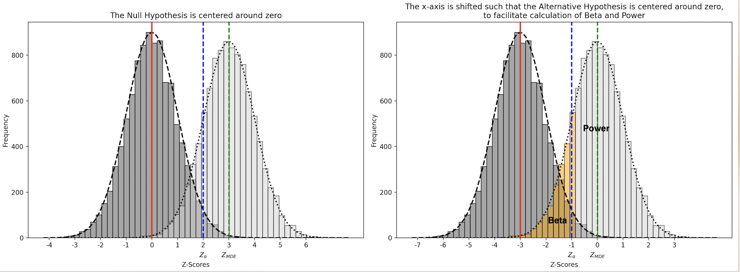
Beta (for a one-tailed test) is therefore calculated as:
\[\beta = P\left(z < z_{\alpha} - z_{\text{MDE}}\right)\]And the corresponding Statistical Power is:
\[\text{Statistical Power} = 1 - \beta = 1 - P\left(z < z_{\alpha} - \frac{\text{MDE}}{\sqrt{\frac{s^2_{\text{test}}}{n_{\text{test}}} + \frac{s^2_{\text{control}}}{n_{\text{control}}}}}\right)\]Given that Statistical Power is conventionally fixed at 80% and alpha is set to 0.05, we can examine the relationship between MDE and the number of samples for a given sample standard deviation \( s \) in the accompanying chart.
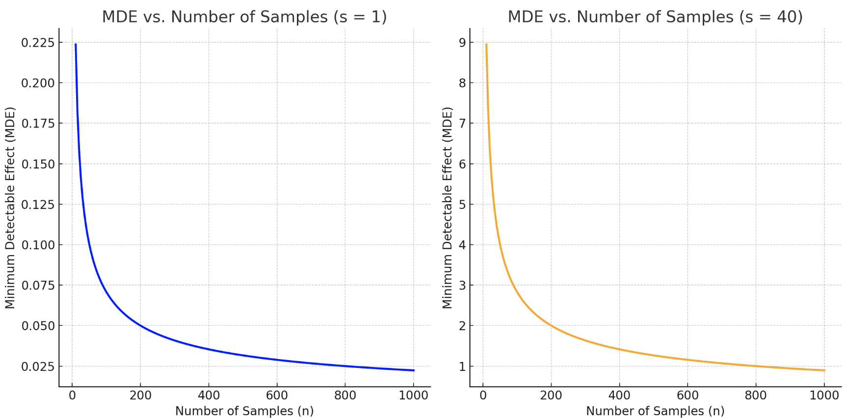
Note that for a two-tailed test, the formula for beta changes to the below i.e. the alpha is halved to account for both tails of the Null Hypothesis.
\[\beta = P\left(z < z_{\alpha/2} - z_{\text{MDE}}\right)\]Although not shown, in this case, the Statistical Power and the relationship between MDE and number of samples would also change accordingly.
Two Sample z-test for Proportions
This is essentially the same as the two-sample z-test for means, in the sense that it deals with independent groups, requires the sampling distribution to be normal, and determines how extreme the observed data is with respect to the distribution under the Null Hypothesis, by calculating the z-statistic and p-value.
The only difference is that this test deals with proportions in categorical data—specifically binary outcomes (e.g., success/failure)—while the other uses continuous data for calculating means. Whereas the z-test for means is used for testing differences in GMV/visitors, the proportions test is used for testing differences in conversion rates.
A Quick Note on Proportions, Ratios, and Means:
As an aside, proportions, ratios, and means are often conflated with each other. These are related but different concepts. Proportions represent part of a whole—they are a fraction or percent. Ratios are a comparison or relationship between data—the data can be unrelated and do not have to form part of a whole. Notably, a proportion can be expressed as a ratio, but a ratio is not a proportion. Means are a summary of the distribution of data, i.e., a summary of a series of values to understand what is the “typical” value. This is in contrast to proportions or ratios that involve the division of one quantity by another. We could take the ratio of means (e.g., mean height of women/mean height of men) or the mean of ratios (e.g., mean of height/weight for women); however, these serve different analytical purposes. The ratio of means shows a relationship between two groups, while the mean of ratios provides a summary within a group—each offering distinct insights depending on the context.
Application of the Central Limit Theorem (CLT) to Proportions:
It was mentioned in the case of the z-test for means that the CLT guarantees that the sampling distribution of means approximates a normal distribution, which in turn allows us to use the z-test. On the other hand, it was mentioned earlier that the CLT does not necessarily apply to all statistics—medians and percentiles being examples.
To clarify, the CLT does indeed apply to proportions. This is because proportions can be modeled as the mean of a series of binary outcomes from a binomial distribution. Under the CLT, the sampling distribution of these means (proportions) from a binomial distribution approximates a normal distribution as the sample size increases, enabling us to apply the z-test.
But going back to the two-sample z-test for proportions, the formula for calculating the standard error, and therefore the z-statistic, looks slightly different from what was used in the case of means, as shown below.
Standard Error for the Difference in Proportions:
By definition:
\[\text{Standard Error} = \sqrt{\text{Var}(\bar{X}_{\text{test}} - \bar{X}_{\text{control}})}\]Because the two samples are independent, the variance of the difference is the sum of the variances of each sample mean:
\[\text{Standard Error} = \sqrt{\text{Var}(\bar{X}_{\text{test}}) + \text{Var}(\bar{X}_{\text{control}})}\]Substituting the variances of the sample proportions, we use \( p_{\text{test}} \) and \( p_{\text{control}} \) to represent the sample proportions for the test and control groups, respectively:
\[\text{Standard Error} = \sqrt{\frac{p_{\text{test}}(1 - p_{\text{test}})}{n_{\text{test}}} + \frac{p_{\text{control}}(1 - p_{\text{control}})}{n_{\text{control}}}}\]Where:
- \( p_{\text{test}} = \frac{x_{\text{test}}}{n_{\text{test}}} \) is the proportion of successes in the test group, where \( x_{\text{test}} \) is the number of successes in the test group, and \( n_{\text{test}} \) is the size of the test group.
- \( p_{\text{control}} = \frac{x_{\text{control}}}{n_{\text{control}}} \) is the proportion of successes in the control group, where \( x_{\text{control}} \) is the number of successes in the control group, and \( n_{\text{control}} \) is the size of the control group.
Pooled Estimate:
Under the Null Hypothesis, we assume that the true proportions in both groups are equal, so we use a pooled estimate \( \hat{p} \), calculated as:
\[\hat{p} = \frac{x_{\text{test}} + x_{\text{control}}}{n_{\text{test}} + n_{\text{control}}}\]Using \( \hat{p} \), the standard error formula becomes:
\[\text{Standard Error} = \sqrt{\frac{\hat{p}(1 - \hat{p})}{n_{\text{test}}} + \frac{\hat{p}(1 - \hat{p})}{n_{\text{control}}}}\]We can then factor out \( \hat{p}(1 - \hat{p}) \):
\[\text{Standard Error} = \sqrt{\hat{p}(1 - \hat{p}) \left( \frac{1}{n_{\text{test}}} + \frac{1}{n_{\text{control}}} \right)}\]Z-statistic for the Difference in Proportions:
As before, the z-statistic is calculated by dividing the observed difference by the standard error, to measure how many standard errors the observed difference is from the expected difference under the Null Hypothesis. Below is the formula for the Statistical Power of a one tailed test.
\[Z = \frac{p_{\text{test}} - p_{\text{control}}}{\sqrt{\hat{p}(1 - \hat{p}) \left( \frac{1}{n_{\text{test}}} + \frac{1}{n_{\text{control}}} \right)}}\]Statistical Power:
The formula for Statistical Power in the case of the difference in proportions is fundamentally similar to that in the case of the difference in means:
\[\text{Statistical Power} = 1 - \beta = 1 - P\left(z < z_{\alpha} - z_{\text{MDE}}\right)\]However, due to the difference in how the standard error is calculated for proportions, the formula becomes:
\[\text{Statistical Power} = 1 - P\left(z < z_{\alpha} - \frac{\text{MDE}}{\sqrt{\hat{p}(1 - \hat{p}) \left( \frac{1}{n_{\text{test}}} + \frac{1}{n_{\text{control}}} \right)}}\right)\]Where:
- \( \hat{p} \) represents the pooled proportion, calculated as:
- \( \text{MDE} \) is the Minimum Detectable Effect, expressed as the difference in proportions you want to detect.
Once again note that the formula for a two-tailed test would be:
\[\text{Statistical Power} = 1 - \beta = 1 - P\left(z < z_{\alpha/2} - z_{\text{MDE}}\right)\]Other Hypothesis Tests
So far, we have covered two variants of the Z-test: the two-sample Z-test for means and the two-sample Z-test for proportions. However, there are other variations of the Z-test, such as the one-sample Z-test (where instead of a Test and Control group, a single group is compared to some specified threshold) and the paired Z-test (where instead of independent Test and Control groups, the group being measured is related in some way). Beyond the Z-test, there are also various other types of hypothesis tests—some that don’t rely on assumptions about the sampling distribution, and others that allow us to assess changes across multiple variables.
Next, we will explore a hypothesis test that measures differences in medians. This test is valuable because medians, being more robust to outliers than means, are an important statistic. Additionally, the test provides a contrast to the z-test.
Mann-Whitney U Test
This test tells us if there is a statistically significant difference between the distributions of two samples (i.e. between the Test and Control groups). And from that, we in turn infer if the difference in medians of the two samples are statistically significant.
Unlike the z-test, this test does not require the sampling distribution to be normal, or make any other assumptions on the sampling or population distributions. In fact this particular test does not even work directly with the data. Instead, it works by comparing the relative rank of the data across the groups.
Under the Null Hypothesis, the expectation is that there is no difference between the two groups—implying that the ranks are randomly distributed between the groups. Deviations from this expectation are also assessed based on the ranked data; although for large samples, these deviations can be further transformed into z-scores for comparison to a normal distribution. The specifics of all this will be illustrated below using an example. The Mann-Whitney test is applicable to continuous or ordinal data. Due to its applicability to continuous data, we can in fact once again leverage our item recommendation module example.
Let us imagine we have 6 visitors in the Control group who are exposed to the old module and 6 visitors in the Test group who are exposed to the new module. The GMV/visitor for each visitor in each group is illustrated below.

As mentioned, the test involves pooling the observations from the two samples into one combined sample, keeping track of which sample each observation comes from, and then ranking lowest to highest from 1 to \(n_{\text{control}} = n_{\text{test}}\), respectively.

Next we compare the sum of each sample’s across-group rank to its within group rank.

A data point’s across-group rank is higher than its within-group rank when a lower-valued data point exists in the other group (which pushes the given data point to a higher rank). The difference between the sum of across-group and within-group ranks reflects the number of times the other group’s values are smaller than those in the given group. This difference effectively measures how much one group’s values tend to be larger than the other’s.
So for instance, the GMV/Visitor datapoint of 11.3 in the Control group has an across-group rank of 4 but a within-group rank of 3 because when the samples are combined, there is one Test group datapoint i.e. 11.0 that is lower than that Control group datapoint.
Similarly the datapoint of 11.5 in the Control group has an across-group rank of 6 but a within-group rank of 4, because there are two Test group datapoints – 11.0 and 11.4 that are smaller than the Control group datapoint. In this way there are 11 instances when the Test group datapoint is smaller than the Control group datapoint, as reflected in the U Statistic of 11 for the Control group.
In this way, there are 11 instances where the Test group’s data point is smaller than the Control group’s, reflected in the U Statistic of 11 for the Control group.

The U Statistic for the Test group is 25, implying that there are 25 instances where there is a Control group datapoint smaller than a Test group datapoint.
To summarize, the formula for the U Statistic is (using the Control group for example):
\[U_{\text{control}} = R_{\text{control}} - \left(n_{\text{control}} \times \left(n_{\text{control}} + 1\right)\right)/2,\]where \(R_{\text{control}}\) is the sum of the across-group rank of the Control data and \(\left(n_{\text{control}} \times \left(n_{\text{control}} + 1\right)\right)/2\) is the sum of the within-group rank of the Control data, derived using arithmetic mean.
The U statistic can be thought of as a rank-based measure of separation between two distributions. Under the null hypothesis, we assume there is no difference between the Test and Control distributions, which implies that, on average, half of the values in one group will rank higher than those in the other group.
To determine statistical significance, we use the smaller of the two U statistic values and compare it to the expected distribution under the null hypothesis. For small samples, this involves comparing the U statistic to a critical value from the Mann-Whitney distribution table, which gives an exact p-value.
It’s important to note that the choice of the smaller U value is purely a matter of convention. The two U statistics are symmetric (i.e., \(U_{\text{control}} + U_{\text{test}} = n_{\text{control}} \times n_{\text{test}}\)), meaning they carry the same information. However, Mann-Whitney tables are designed for comparison using the smaller U statistic.
For larger samples, it becomes computationally impractical to create a distribution table for exact p-values. In such cases, we leverage the Central Limit Theorem (CLT). While the CLT is often associated with the convergence of sample means to a normal distribution for large samples, it more generally states that for independent and identically distributed (i.i.d.) large samples, the scaled sum of the data (which includes the mean but not the median or percentiles) converges to a normal distribution.
The U statistic, being based on the sum of across-group ranks and within-group ranks, fits this framework. Thus, for large samples, the CLT guarantees that the U statistic approximates a normal distribution.
Any U statistic can therefore be converted to a z-score and compared to the normal distribution under the null hypothesis to assess how extreme the observed value is. As mentioned earlier, under the null hypothesis, we expect half the values in one group to be higher than that in the other group. It was also mentioned that \(U_{\text{control}} + U_{\text{test}}\) is always \(n_1 \times n_2\). Given this, the mean value under the Null Hypothesis is \((n_1 \times n_2)/2\)
Additionally, the standard deviation of the U statistic under the null hypothesis is given by:
\[\sigma_U = \sqrt{\frac{n_1 \times n_2 \times (n_1 + n_2 + 1)}{12}}\](Note that the formula for standard deviation changes when there are ties in the rankings to
\[\sigma_U = \sqrt{ \frac{n_1 \times n_2 \times (n_1 + n_2 + 1)}{12} - \frac{\sum_{i} (t_i^3 - t_i)}{12(n_1 + n_2)(n_1 + n_2 - 1)} }\]Where \( t_i \) is the number of tied ranks in the \( i \)-th group of ties. However, further details on this are beyond the scope of this discussion.)
The z-score of the U statistic is then calculated as:
\[Z = \frac{U - \mu_U}{\sigma_U}\]This z-score can be compared to the standard normal distribution to determine statistical significance.
Note that, it was mentioned earlier that using the smaller U was a matter of convention, necessary when finding exact p-values from the Mann-Whitney distribution table. In contrast, for large samples, either of the U Statistic yields the same p-value.
In our example, we get \(\mu_U = 18\), and \(\sigma_U = 6.244\). Since \(U_{\text{control}} = 11\) and \(U_{\text{test}} = 25\), we get
\[Z_{\text{control}} = \frac{11 - 18}{6.244} \approx \frac{-7}{6.244} \approx -1.12\]and
\[Z_{\text{test}} = \frac{25 - 18}{6.244} \approx \frac{7}{6.244} \approx 1.12\]As can be seen above, the two U Statistics yield symmetric z-scores and therefore the same p-value i.e. 0.2623 (which is not statistically significant).
Note, the sample sizes in our example (\n_(\text{control} = n_{\text{test}} = 6\)) are too small to use the Z-score approach accurately. The rule of thumb is that we require at least 30 samples for the z-score based approach to apply. However, the above is intended to illustrate the symmetry in z-scores which still holds for larger sample sizes, where the normal approximation becomes valid.
A Disclaimer on Inferring Medians:
The Mann-Whitney U test can detect differences between distributions, but it does not automatically imply that the medians are different unless the two distributions have the same shape. Differences in the overall shape of the distributions (e.g., spread or skewness) can also lead to a rejection of the null hypothesis, even when the medians are the same.
This is an important caveat when using non-parametric tests like Mann-Whitney, as they test for differences in ranks and distributions rather than focusing solely on central tendencies like the median.
For example, in the image below, the medians of both distributions are identical. However, the null hypothesis would still be rejected in this case because the distributions are skewed in different directions.
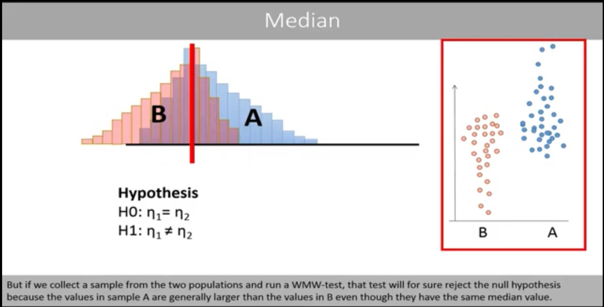
Image Source: The Mann Whitney U test (Wilcoxon Mann Whitney test)
In short, the Mann-Whitney test can tell us if the distributions of two groups are different. However, it does not necessarily indicate that the medians of the distributions are different unless the distributions have the same shape. Inferring that the medians are different would require the additional assumption that the distributions are similarly shaped.
This is why Mann-Whitney tests are often reported as stating: “The medians of the two groups were different, and there was a statistically significant difference detected between the two groups,” as opposed to “The medians of the two groups were statistically significantly different.”
Statistical Power:
The statistical power calculation for the Mann-Whitney test is not as straightforward as that for z-tests. For small samples, a formula-based power calculation is generally not possible due to the non-normality of the U statistic’s distribution. In these cases, we rely on Monte Carlo simulations or exact methods to estimate power (Monte Carlo is to be discussed in a later section).
For large samples, we can use the asymptotic normal approximation of the U statistic, similar to the z-test, to calculate power. However, regardless of sample size, the MDE (Minimum Detectable Effect) for the Mann-Whitney test must be handled with care.
In z-tests, the MDE is typically defined as a difference in means. In the Mann-Whitney test, since the test compares the ranks of two groups rather than their raw data, it makes sense to approach the MDE as a shift in ranks, which is reflected in the U statistic. However, because the U statistic may not be easily interpretable, we often express the effect size in terms of the probability of superiority, which is a transformation of the U statistic.
The probability of superiority is calculated as:
\[\text{Probability of Superiority} = \frac{U}{n_1 \times n_2}\]This tells us the likelihood that a randomly selected value from the test group will exceed a randomly selected value from the control group, making it an intuitive measure of effect size in the Mann-Whitney test.
An example of power calculation for large sample Mann-Whitney test is as follows (however we will still use our previous example of \(n_{\text{control}} = n_{\text{test}} = 6\), which does not technically apply but enables simpler illustration):
As seen before, in our example \(n_{\text{control}} = n_{\text{test}} = 6\), \(\mu_U = 18\) and \(\sigma_U = 6.244\)
Let us say we want our probability of superiority to be 0.65. Therefore our \(U_{\text{MDE}} = n_{\text{control}} \times n_{\text{test}} \times \text{Probability of Superiority} = 6 \times 6 \times 0.65 = 23.4\)
\[Z_{\text{MDE}} = \frac{U_{\text{MDE}} - \mu_U}{\sigma_u} = 0.865\]In the section for z-test, we have seen that the formula for statistical power for a right tailed test = \(1 - P(Z < Z_{\alpha} - Z_{\text{MDE}})\)
For a one tailed test, the critical value of \(Z_{\alpha}\) for a 5% significance level is 1.64.
\[\left(z_{\alpha} - z_{\text{MDE}}\right) = 1.64 - 0.865 = 0.775\]From Z-tables, the probability of obtaining a Z-score less than 0.775 is approximately 0.78.
Therefore, the power of the test is approximately 1 - 0.78 = 0.22 i.e. 22%
On the other hand, for a two tailed test, the critical value of \(Z_{\alpha/2}\) for an overall 5% significance level is 1.96.
\[\left(z_{\alpha/2} - z_{\text{MDE}}\right) = 1.96 - 0.865 = 1.095\]therefore \(P\left(z < z_{\alpha/2} - z_{\text{MDE}}\right) = 0.863 \)
and Statistical Power = 1 - 0.863 = 0.137 i.e. 13.7%
Family of Hypothesis Tests
There are a very large number of statistical tests depending on data type, sample size, number of groups, test statistic, type of comparison, number of dependent variables and so on. The internet is replete with flow charts that help determine which statistical test is appropriate for a given situation. A couple of these are shared below:
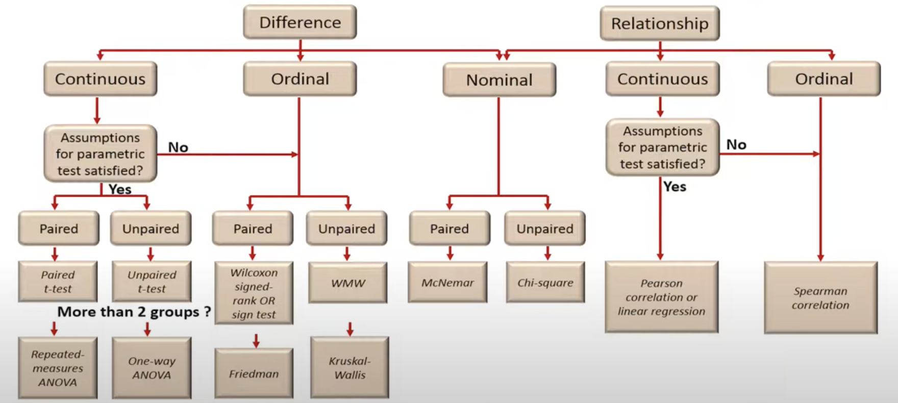
Image Source: How to choose an appropriate statistical test
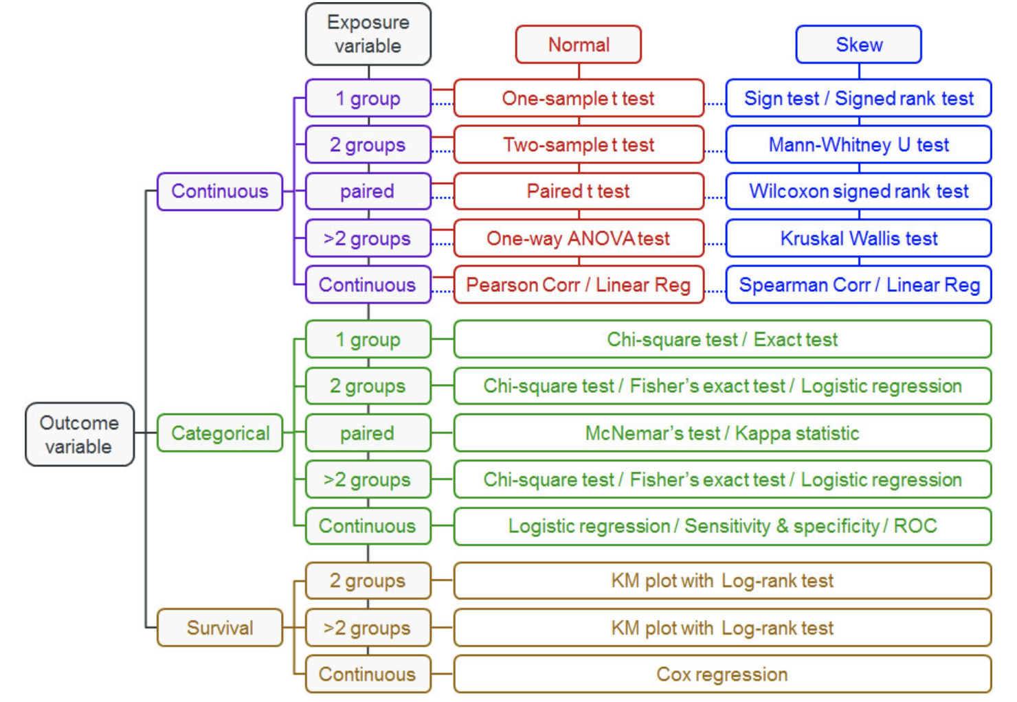
Image Source: Flow chart for Which Statistical Test
Some argue that there is essentially only one statistical test: it involves simulating the expected distribution under the null hypothesis and then evaluating the probability of observing data as extreme as the actual data, given that distribution. Historically, analytical methods like t-tests or chi-square tests were developed because computation was slow and expensive, necessitating exact, formula-driven solutions. However, as computation has become faster and more accessible, these methods, though efficient, have become less appealing due to their rigid assumptions and limited flexibility.
In contrast, simulation-based methods such as permutation tests, bootstrapping, and Monte Carlo simulations are highly flexible. They allow us to model a wide range of scenarios and try different test statistics, making it easier to choose the most appropriate approach for a given problem. By relying on simulations, we can tailor statistical tests to the data at hand, without being constrained by the assumptions required by traditional analytical methods.
In the following sections, we will explore the aforementioned methods and demonstrate how they provide robust alternatives to more traditional techniques.
Permutation Tests
Permutation Tests work by assuming the test and control groups come from the same distribution, which reflects the Null Hypothesis. Under this assumption, if we reshuffle and randomly reassign the data points between test and control groups, the resulting groups are statistically equivalent to the original ones, as they all come from the same underlying distribution. (Note: These reshuffled groups are the same size as the original.)
The difference between the test statistic of the original test/control groups and that of the reshuffled groups is entirely due to sampling variability. The permutation test repeats this reshuffling and recalculation of the test statistic many times to create a Null Distribution of the test statistic.
Finally, the test compares the observed test statistic to this generated null distribution to calculate a p-value, which measures how likely the observed test statistic is under the null hypothesis. This tells us how extreme the observed test statistic is, providing evidence for or against the null hypothesis.
It may be illuminating to see how Permutation Tests work by first considering a test and control group which comes from two well separated distributions and then considering the case where test and control groups come from overlapping distributions.
Case 1: Permutation Test for the mean difference of well-separated distributions
Suppose our Control group follows a normal distribution with mean of 3 and standard deviation of 1, while the test group follows a normal distribution with mean of 8 and standard deviation of 1. These are the true population parameters that we are able to dictate since we are doing a simulation.
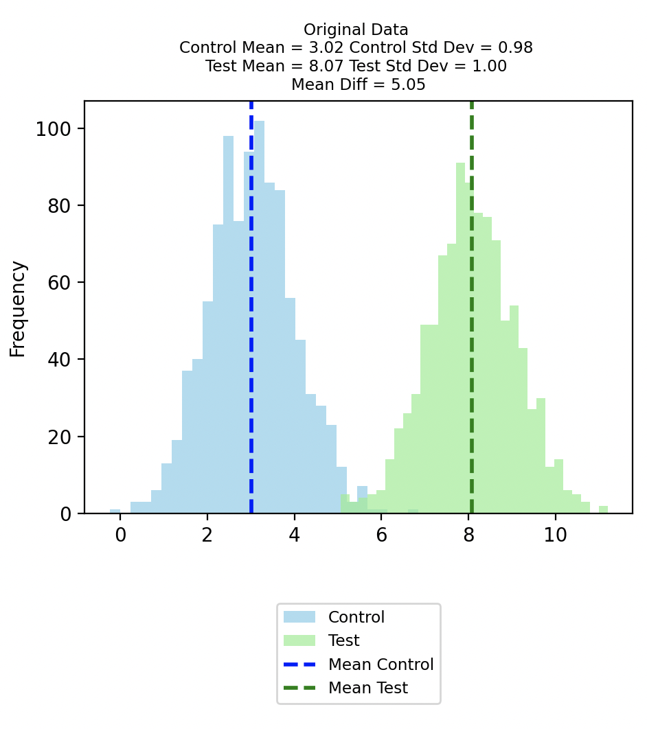
From this population, suppose we draw 1000 samples for test and control groups respectively, and get the distributions below.
This Original Control group has a mean of 3.02 and a standard deviation of 0.98; while this Original Test group has a mean of 8.07 and a standard deviation of 1.00. The difference between the means of the original data is 5.05. Through the Permutation Test we will later ascertain if this difference between the means is statistically significant or not.
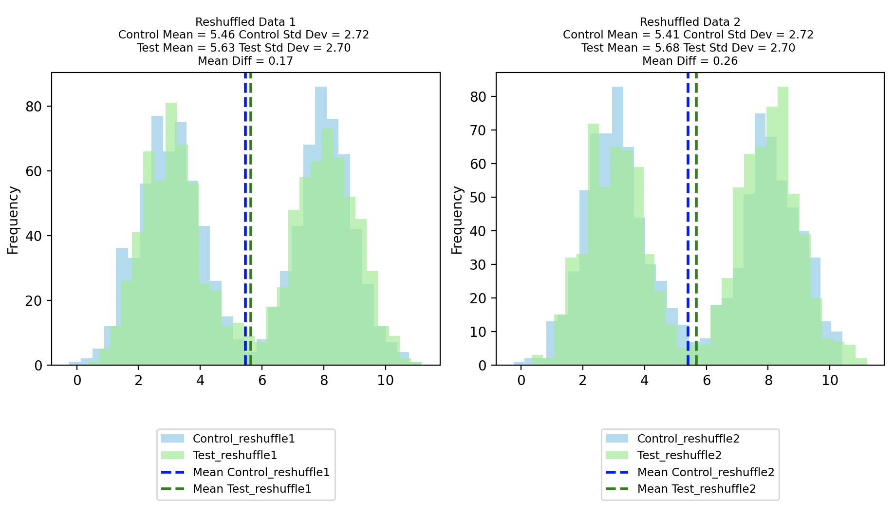
As mentioned, the Permutation Test entails reshuffling the data and randomly assigning them to new Reshuffled Control and Reshuffled Test groups. Below we see distributions for two instances of reshuffling.
In the first reshuffle, we happen to get a Reshuffle 1 Control with mean 5.46 and standard deviation 2.72 and Reshuffle 1 Test with mean 5.63 and standard deviation 2.70, resulting in a mean difference of 0.17
While in the second reshuffle, we happen to get a Reshuffle 2 Control with mean 5.41 and standard deviation 2.72 and Reshuffle 2 Test with mean 5.68 and standard deviation 2.70, resulting in a mean difference of 0.26.
Even though the Reshuffled Control and Reshuffled Test data come from the same distribution by design, their difference in means change due to sampling variability.
(As an interesting aside, note the bimodal distribution of the Reshuffled Control and Reshuffled Test distributions, confirming that they do indeed consist of randomly selected data from the original well separated test and control.)
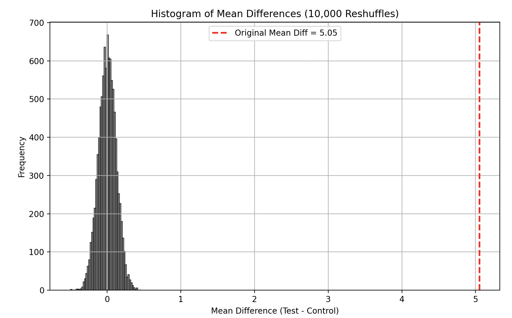
On each reshuffle we are specifically interested in the difference in means between the Reshuffled Test and Control, since we want to create a sampling distribution of the difference in means.
In fact we do a total of 10,000 reshuffles to get the sampling distribution of the difference in means as shown below. The dashed red line indicates our original mean difference, and since it does not overlap at all with the sampling distribution of mean differences, we can say the p-value of our observation is 0 and thus our observation is statistically significant!
Case 2: Permutation Test for the mean difference of overlapping distributions
We now consider the case when the Control and Test groups are not as well separated. This time suppose our true population parameters are as follows: the Control group follows a normal distribution with a mean of 3 and a standard deviation of 40. The Test group follows a normal distribution with a mean of 4 and a standard deviation of 40.
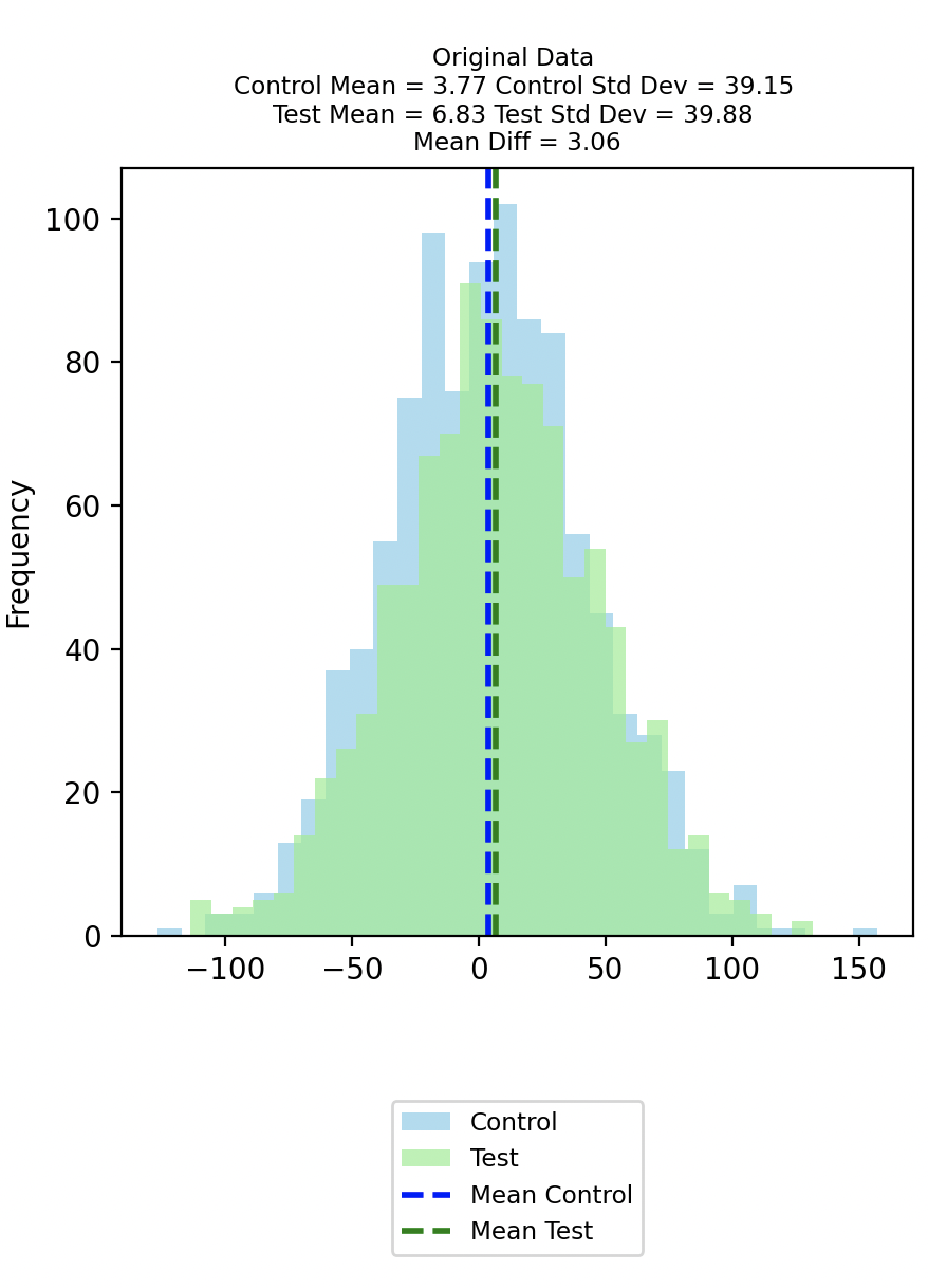
Drawing 1000 samples from the Control and Test populations respectively gives us the distributions in the chart below.
This Original Control group has a mean of 3.77 and a standard deviation of 39.15; while this Original Test group has a mean of 6.83 and a standard deviation of 39.88. The difference between the means of the original data is 3.06.
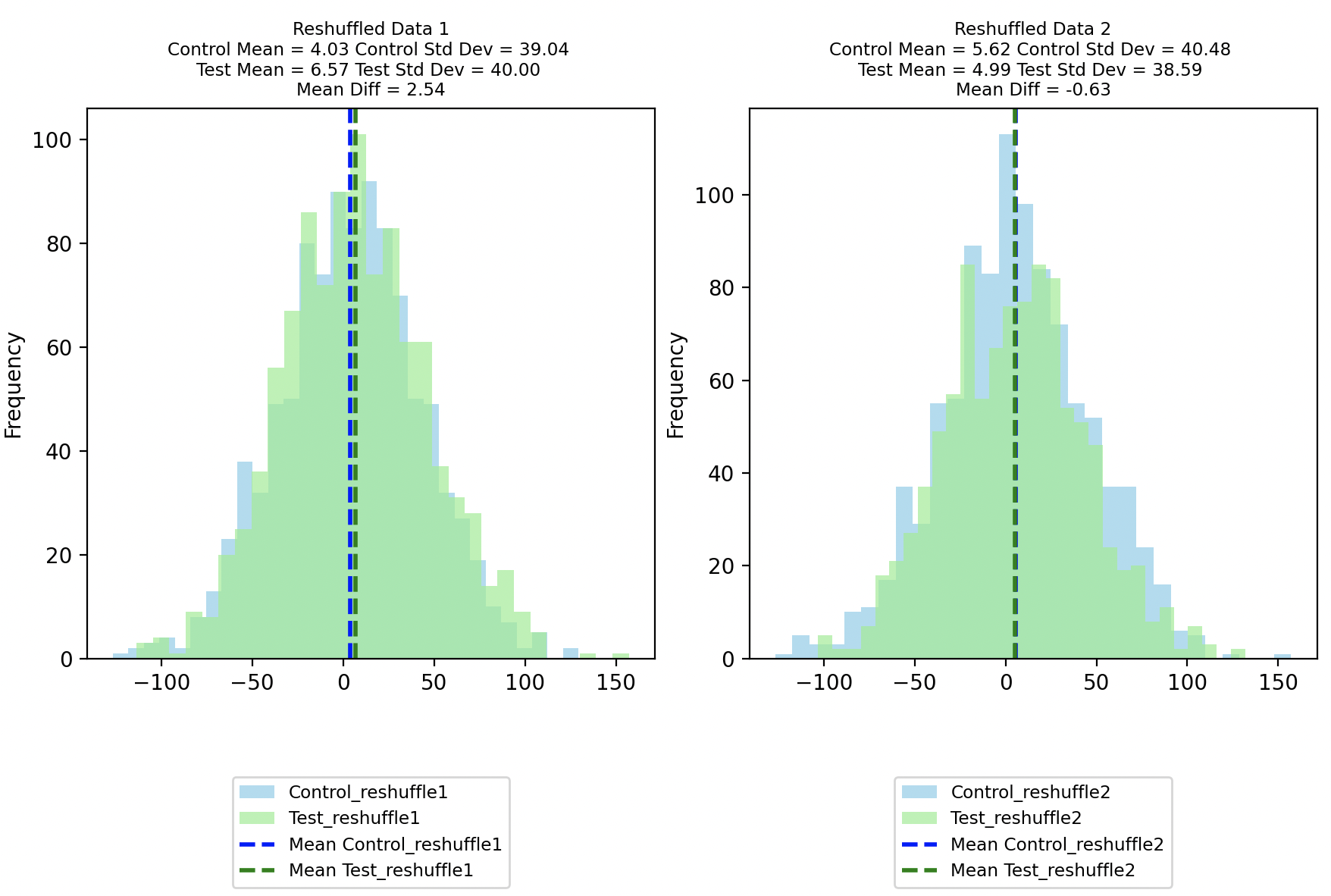
Reshuffling the data does not lead to a bimodal distribution in this case, which is expected since the Original Control and Test distributions overlap. There is however still sampling variability, evident due to the difference in mean being 2.54 in the first shuffle and -0.63 in the second shuffle.
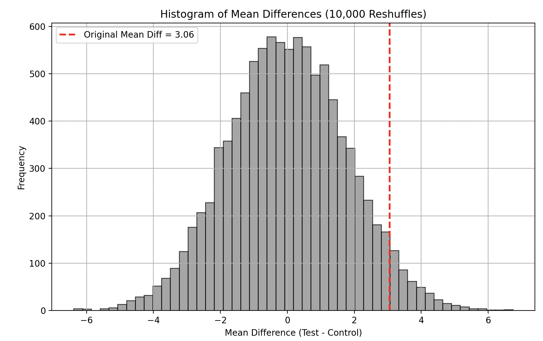
A total of 10,000 reshuffles yields the distribution of mean differences as can be seen in the plot below. Once again, the dashed red line indicates our original mean difference. This time however it does overlap with the sampling distribution of mean differences. To calculate the p-value, we measure the proportion of reshuffled mean differences that are as extreme or more extreme than the original observed mean difference, relative to the total number of reshuffled mean differences. The p-value turns out to be 0.083 in this case indicating that our observation is not statistically significant.
In the examples above, we applied the Permutation Test to assess the difference in means, but it can be similarly applied to test differences in medians. The key assumption of Permutation Tests is that the data are exchangeable (i.e., identically distributed under the null hypothesis) and independent. Consequently, permutation tests may not perform well in cases of small sample sizes, multivariate data, time-series data, heavily skewed distributions, or non-independent data (such as clustered observations).
Note the code for running the permutation tests and generating the associated charts is here.
Bootstrapping (and Confidence Intervals)
Having looked at Permutation Tests, we now turn our gaze on to another simulation method—bootstrapping. In the words of statistician Phillip Good: “Permutations test hypotheses concerning distributions; bootstraps test hypotheses concerning parameters.” So whereas for permutation tests, we assume that under the null hypothesis, the test and control data come from the same distribution, bootstrapping makes no such assumption. Instead, bootstrapping assumes that each group (i.e., sample) represents its respective population. By resampling with replacement from the observed data, bootstrapping allows us to estimate the variability of a statistic (e.g., mean, median, or 90th percentile), providing insights into the population without needing to assume any specific underlying distribution.
Resampling with replacement is fundamental to the concept of bootstrapping. Resampling without replacement would not allow us to maintain the same sample size as the original, which is why bootstrapping relies on resampling with replacement. By keeping the bootstrapped sample sizes consistent with the original, this method mimics the natural variability that occurs when sampling from a population, allowing us to approximate how the statistic would behave if we repeatedly sampled from the population. I do, however, have an open question regarding this process, but I will set it aside for now and revisit it later.
Bootstrapping generates a sampling distribution of a statistic. From this distribution, we can calculate the mean of the statistic (i.e. the mean of the mean, median, or 90th percentile) and determine the range within which 95% of the resampled statistics lie around this mean. This range is known as the confidence interval, and it provides an estimate of the uncertainty around the statistic. Confidence intervals can also be used in hypothesis testing to assess whether a specific value (e.g., a null hypothesis parameter) falls within this range, offering a way to evaluate statistical significance without assuming any specific underlying distribution. All this shall be illustrated through the example below.
Case 1: Bootstrapping for the mean difference of well-separated distributions
In the previous section we had looked at applying the Permutation Test to a Control and Test Distribution drawn from two well separated population distributions.
We revisit the same population and original sampled distribution, but this time we apply bootstrapping to find the distribution of bootstrapped means and the 95% confidence interval around the mean of the bootstrapped mean.
In the chart below, we see the distribution of the bootstrapped sample means overlaid on the original sample distributions. Note we calculate the histograms for the bootstrapped means and then scale their heights to not exceed the max height of the original histograms, making them visually comparable without overshadowing the original data.
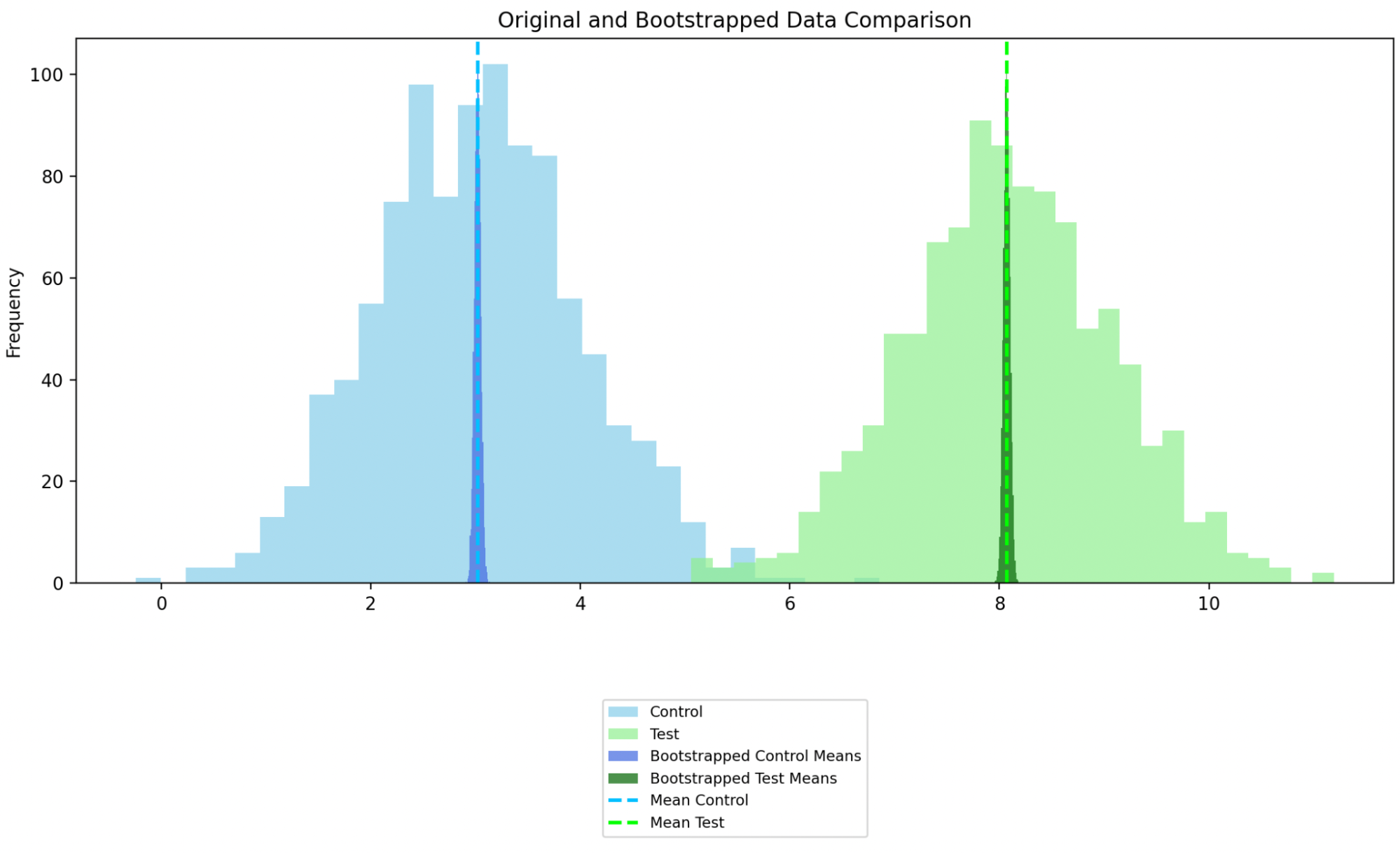
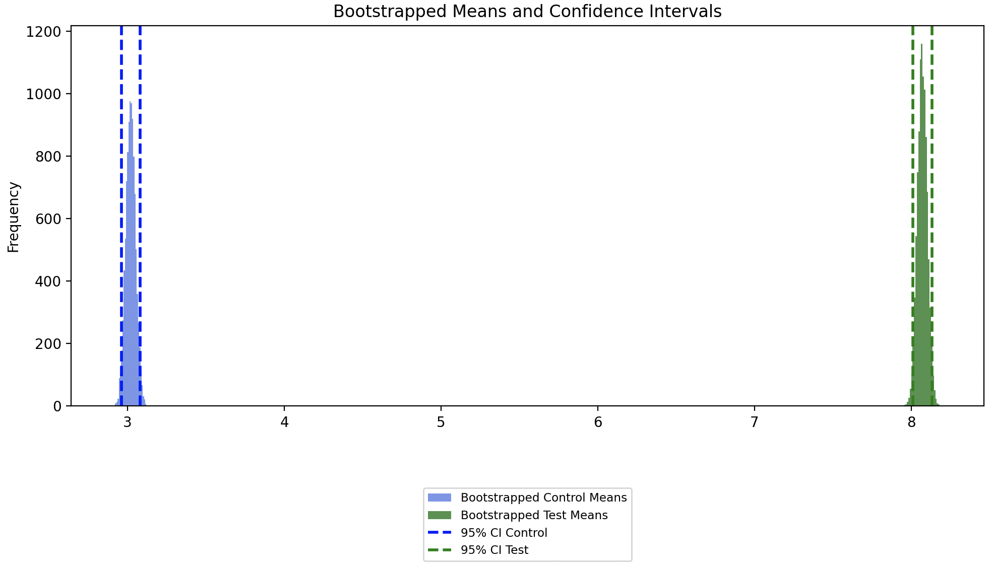
A closer look at the bootstrapped sampled means shows the mean of the bootstrapped means and its 95% confidence intervals. Since the confidence intervals of the bootstrapped Control and Test groups don’t overlap, this indicates that there is a statistically significant difference between the Control and Test groups.
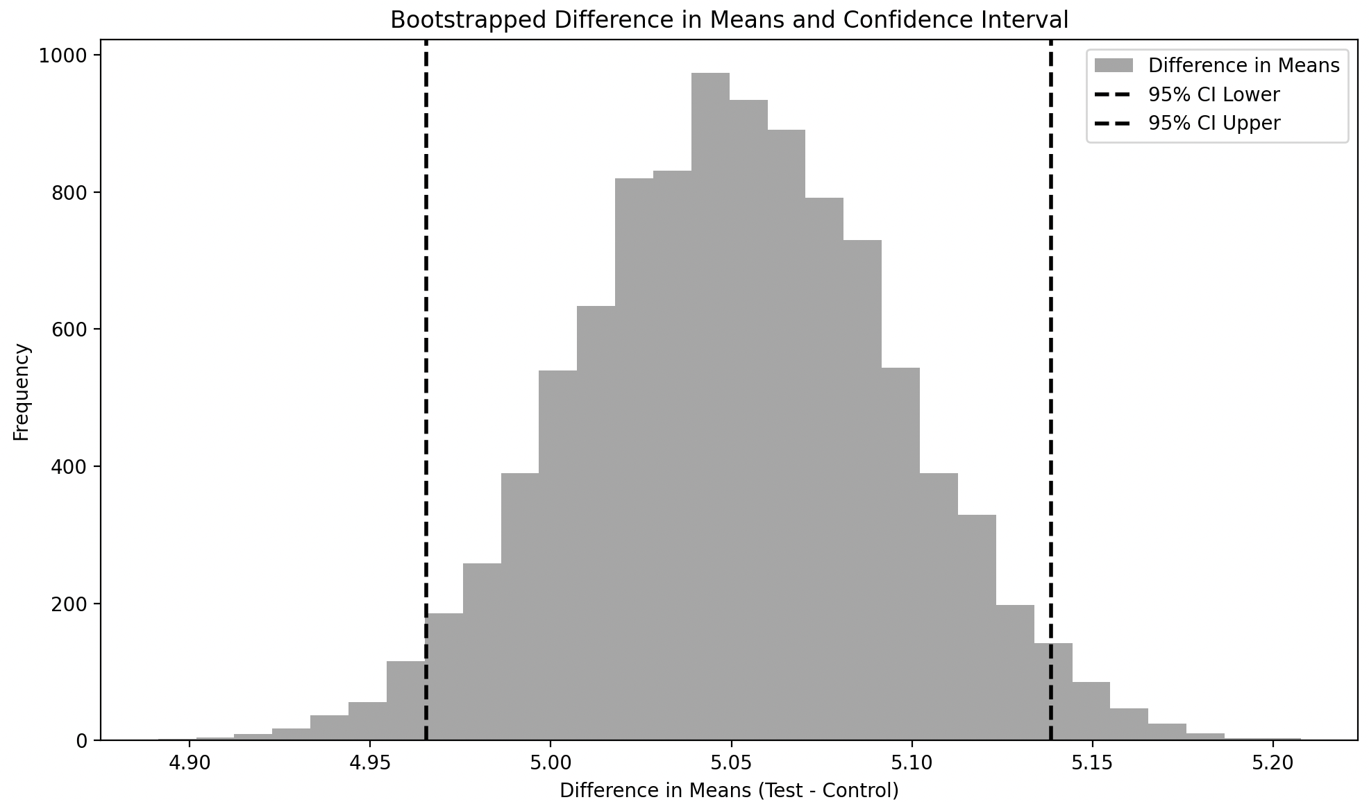
We can also take a look at the distribution of the difference of the bootstrapped sample means along with its mean and confidence interval. The confidence interval of the difference in the means does not include zero, which implies that there is a 95% probability that the difference in means is not zero or only a 5% probability that the difference in means is zero. In short, since the confidence interval of the difference in means does not include zero, we can say that the difference in Test and Control groups is statistically significant
.
Case 2: Bootstrapping for the mean difference of overlapping distributions
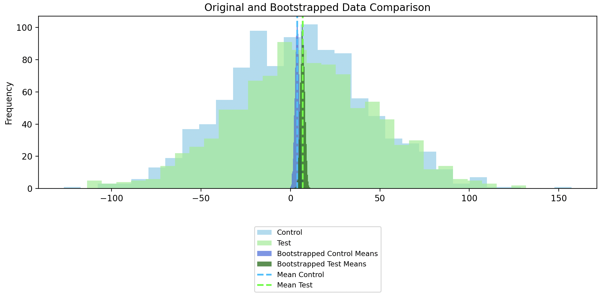
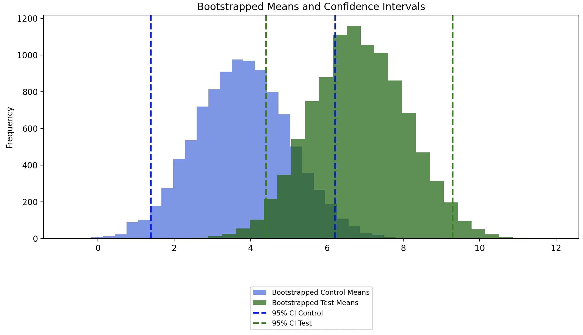
In this case, we can see that the confidence intervals of the bootstrapped Control and Test groups overlap, which indicates that there* isn’t* a statistically significant difference between the original Control and Test groups.
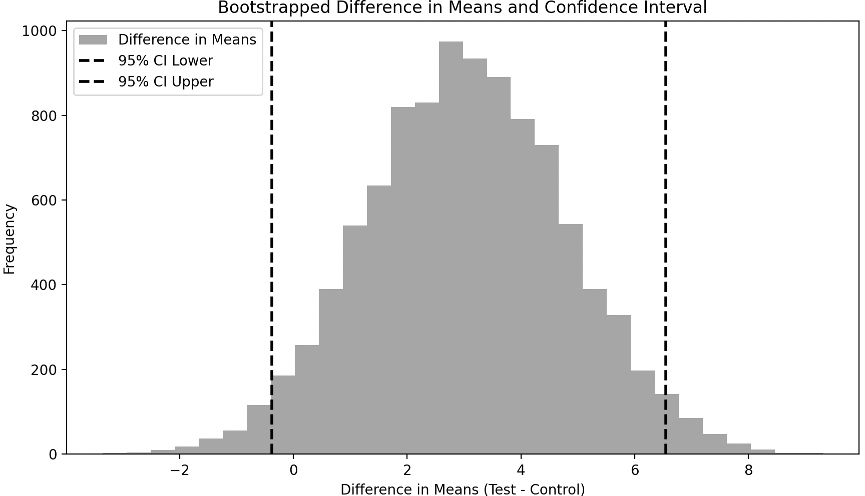
We can also see that the confidence interval around the difference of the bootstrapped sample means includes zero, meaning that the difference between the Control and Test groups is not statistically significant.
Note that the results of bootstrapping is consistent with what we saw using Permutation Tests for Case 1 and 2 respectively. Also note the code for bootstrapping means and generating the associated charts is here.
Case 3: Bootstrapping for the 90th percentile difference of overlapping distributions
So far we have considered means as our statistic of interest just to illustrate how bootstrapping works. However bootstrapping is most useful when calculating statistics like percentiles, as mentioned earlier.
To illustrate bootstrapping for the difference in the 90th percentile, let us consider the overlapping distributions from Case 2.
In the chart below, we see the distribution of the 90th percentiles of bootstrapped samples overlaid on the original sample distributions. Once again, the distribution of the 90th percentiles of bootstrapped samples are scaled down to not exceed the height of the original sampled distributions, for easier comparison.
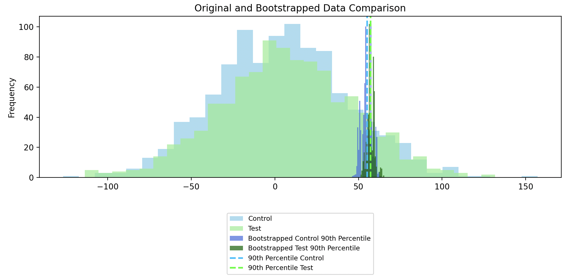
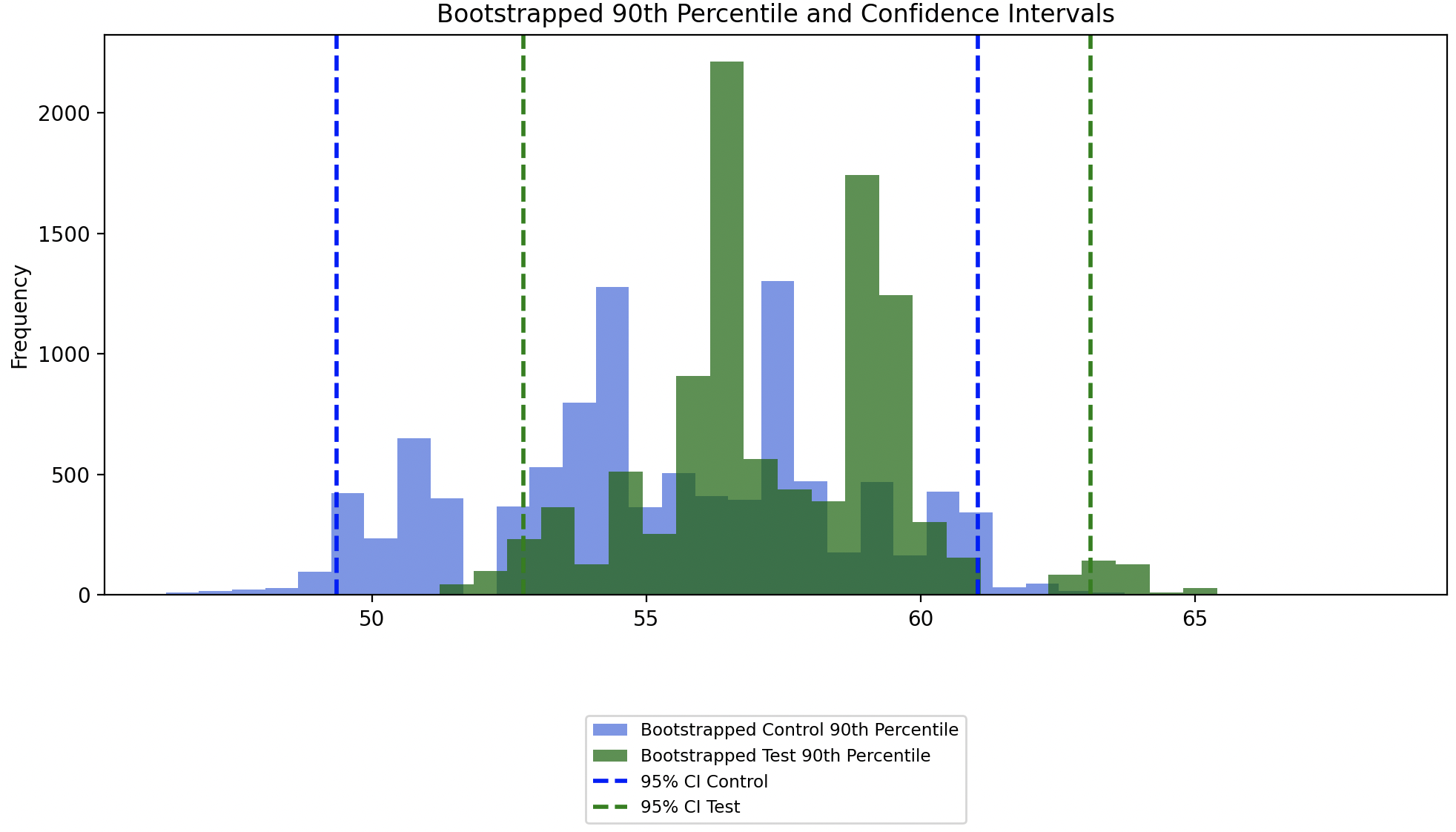
Since the confidence intervals of the 90th percentile of the bootstrapped Control and Test groups overlap, this indicates that there isn’t a statistically significant difference between the 90th percentile of the original Control and Test groups.
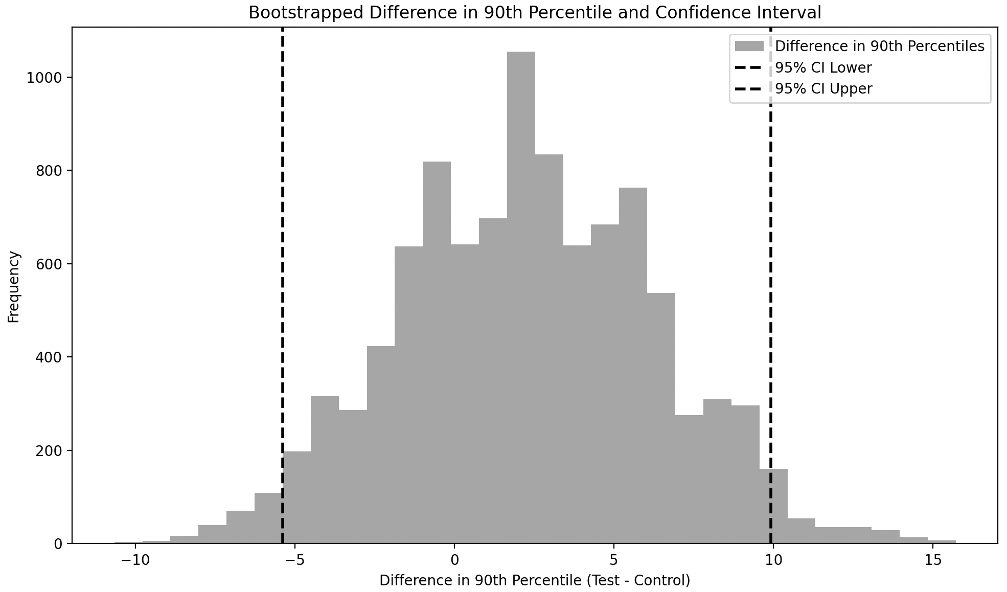
The confidence interval around the difference of the 90th percentile of bootstrapped samples includes zero, meaning that the difference between the 90th percentile of the Control and Test groups is not statistically significant.
The code for bootstrapping means and generating the associated charts is here.
Sampling with replacement or without replacement
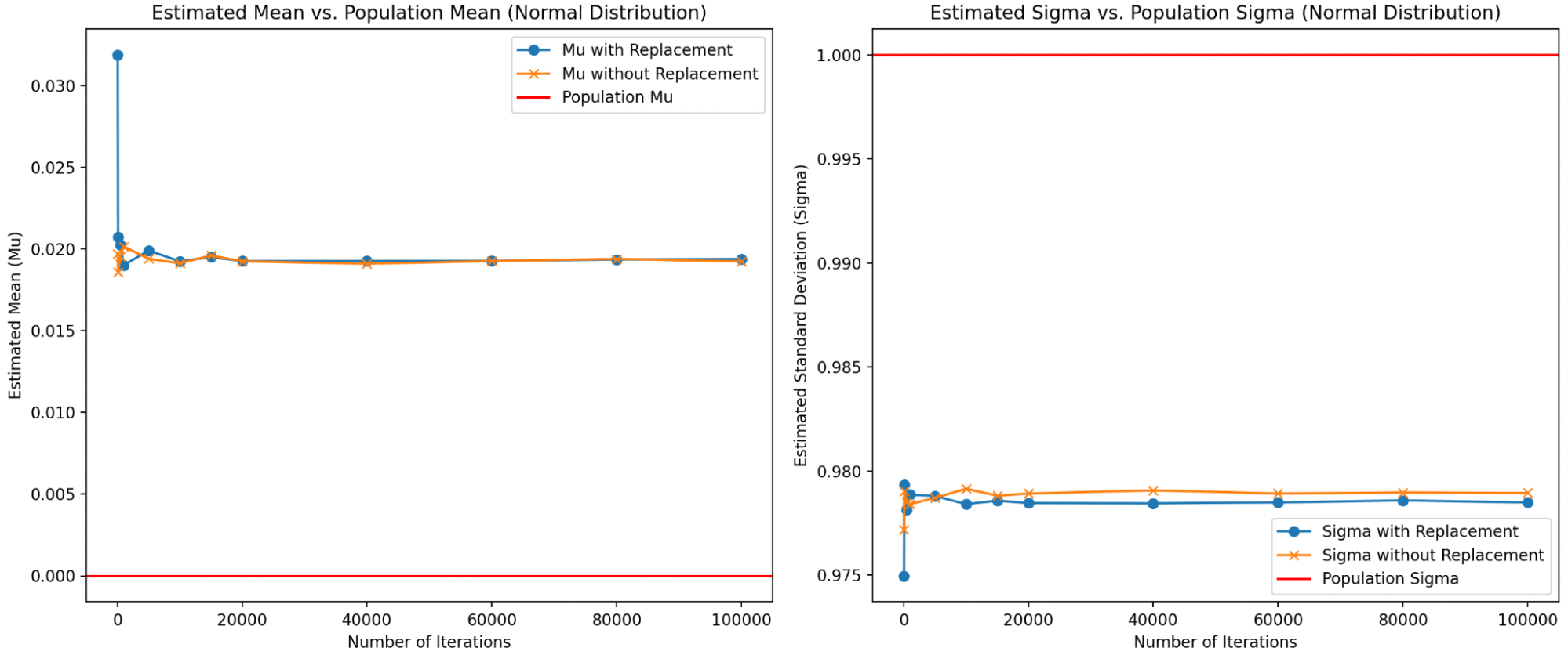
As mentioned, bootstrapping requires sampling with replacement to maintain consistency in sample size with the original dataset. However, an interesting question arises: why must the sample size remain consistent? Could we not use a smaller sample size for each iteration and compensate by increasing the number of iterations?
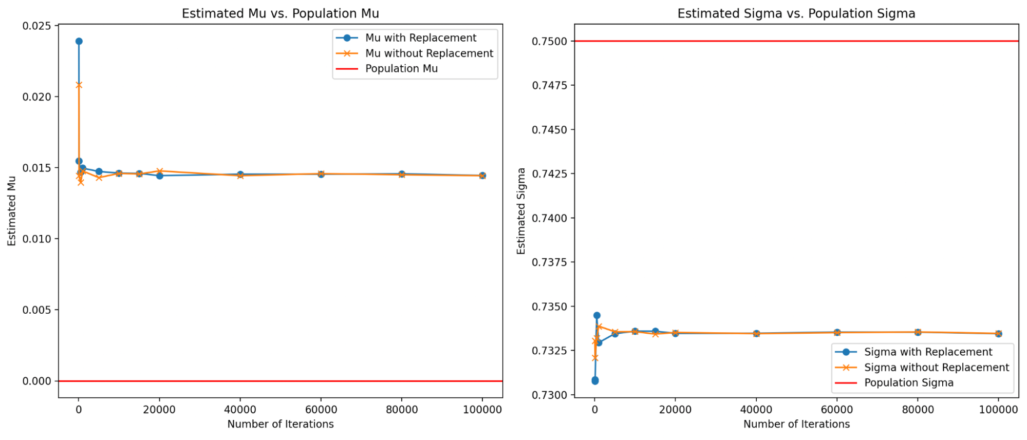
Below, I explore this idea and show that, at least for the normal, lognormal and exponential distributions, reducing the sample size and then sampling without replacement actually produces reasonable results even for low iterations.
Comparison of parameter estimation for the Normal distribution using bootstrapping with and without replacement:
Comparison of parameter estimation for the Lognormal distribution using bootstrapping with and without replacement:
Comparison of parameter estimation for the Exponential distribution using bootstrapping with and without replacement:
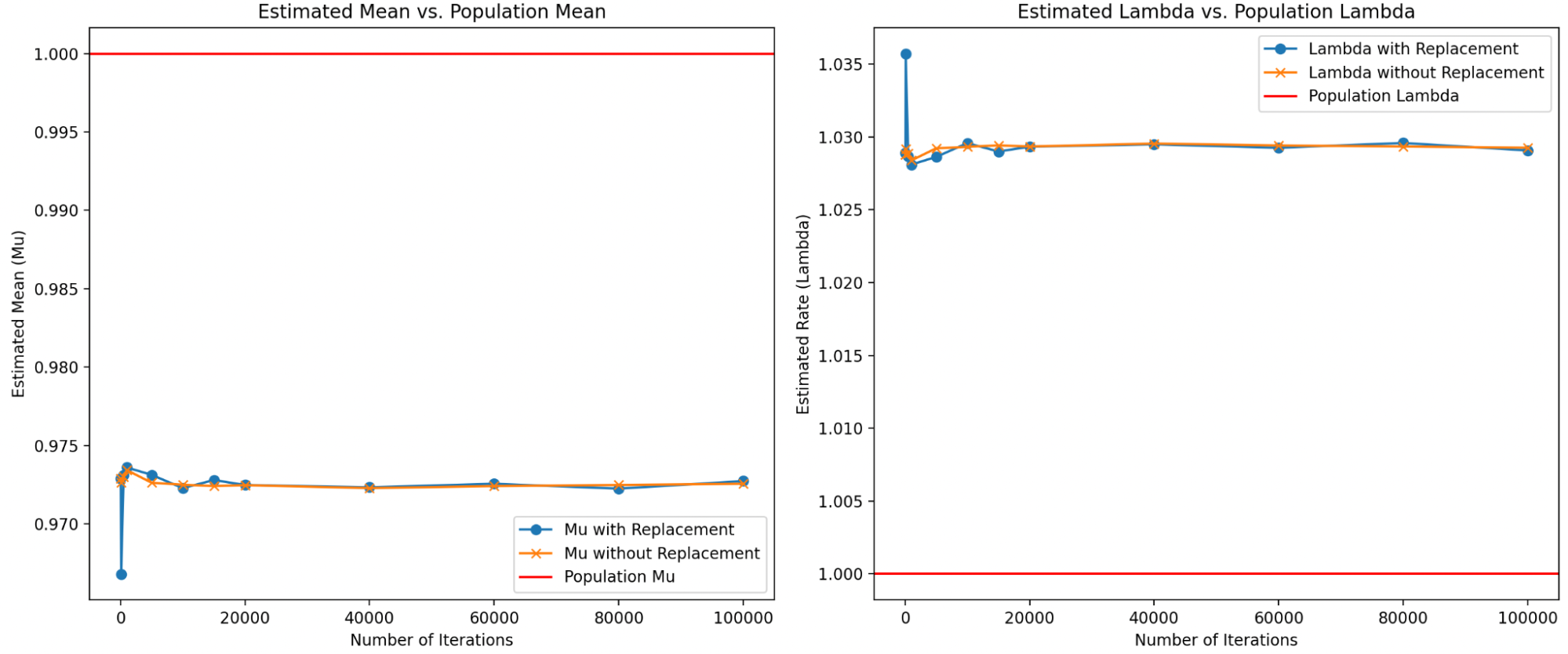
For now, I’ll adhere to the traditional approach of bootstrapping with replacement, which ensures sample size consistency and minimizes bias across a range of distributions. But the results of this simulation are compelling, and I plan to explore the implications of reduced sample size in more detail later.
The code for sampling with or without replacement is here.
Monte Carlo
Monte Carlo works by generating synthetic data according to known rules. Sometimes these rules may not be exactly known, but we still make an assumption for the purpose of data generation. The assumption doesn’t have to be correct in the real world but is used to approximate how the test behaves under certain conditions.
So in contrast to Permutation tests, which assume that both the test and control groups come from the same distribution, and Bootstrapping, which assumes the observed data is representative of the population, Monte Carlo methods aim to mimic the data-generating process itself. By generating synthetic data, we can analyze the resulting statistics and relationships of interest.
As mentioned earlier, Monte Carlo methods are used to calculate statistical power for small samples in the Mann-Whitney test. This will be illustrated by revisiting the example from the Mann-Whitney test section where we considered sample size of 6 for both test and control group, as well as a probability of superiority of 65%.
We perform Monte Carlo as follows:
- Generate Distributions: We first create two distributions reflecting the stated probability of superiority.
- Repeated Testing: We then conduct the Mann-Whitney U test multiple times (for example, 10,000 iterations), using randomly selected groups of six samples from each distribution.
- Evaluate Power: We assess the proportion of these tests where the null hypothesis (that the distributions are identical) is rejected. This provides an estimate of the test’s power.
It’s important to note that while we assume the generated distributions are normal for simplicity, the Monte Carlo method can be adapted to work with any type of distribution.
The code for the test is as follows:
import numpy as np
import scipy.stats as stats

def generate_data(n_control, n_test, prob_superiority):
    # Control group: Standard Normal Distribution
    control = np.random.normal(0, 1, n_control)
    # Test group: Shifted distribution based on probability of superiority
    # Finding the required shift using the inverse of the cumulative distribution function
    shift = stats.norm.ppf(prob_superiority)
    test = np.random.normal(shift, 1, n_test)
    return control, test

def perform_mann_whitney(control, test):
    # Perform Mann-Whitney U test
    u_stat, p_value = stats.mannwhitneyu(control, test, alternative='two-sided')
    return p_value

def monte_carlo_simulation(n_control, n_test, prob_superiority, n_simulations=10000, alpha=0.05):
    significant_count = 0
    for _ in range(n_simulations):
        control, test = generate_data(n_control, n_test, prob_superiority)
        p_value = perform_mann_whitney(control, test)
        if p_value < alpha:
            significant_count += 1
    return significant_count / n_simulations

# Simulation parameters
n_control = n_test = 6
prob_superiority = 0.65
n_simulations = 10000
alpha = 0.05  # Significance level

# Run Monte Carlo simulation
power = monte_carlo_simulation(n_control, n_test, prob_superiority, n_simulations, alpha)
print(f"Estimated power of the test: {power:.4f}")
Running the above tells us that the Statistical Power will be 0.072, whih is actually half of the power suggested by using the formula. However as was mentioned earlier, due to the sample sizes being very small the formulaic approach does not quite apply here; therefore this Monte Carlo method is a better approximation of the statistical power.
An adjacent example for using Monte Carlo to calculate the minimum sample size is in this excellent video
Wrapping it up
This essay covered the central concepts of Hypothesis Testing such as sampling variability, sampling distributions, statistical significance, Null and Alternative Hypothesis, statistical power, Type 1 and 2 errors, the Central Limit Theorem and the Law of Large Numbers. It then illustrated these concepts with specific tests such as z-tests for means and proportions, Mann-Whitney test; as well as simulation methods like Permutation Tests, Bootstrapping and Monte Carlo.
However we have only considered univariate tests. Multivariate tests will be explored in a future essay. There are also related concepts such as handling outliers, p-hacking, time to run tests, internal and external validity that will be tackled in future essays.